Chapter 2 Stochastic shortest path problems

With the basic MDP framework as described in the previous chapter, we consider the following infinite horizon cost objective for any policy \(\pi\) and initial state \(x_0\): \[\begin{align} J_\pi(x_0) = \lim_{N\rightarrow\infty} \mathbb{E}\left[ \sum_{k=0}^{N-1} \alpha^k g(x_k, \mu_k(x_k), x_{k+1}]\right], \tag{2.1}\end{align}\] where \(\alpha \in (0,1]\) is a discount factor. The goal is to find a policy \(\pi^*\) that solves the following problem: \[\min_{\pi \in \Pi} J_\pi(x_0),\] where \(\Pi\) is a subset of admissible policies, that satisfies certain conditions based on the underlying model. We study the following models under the objective defined above:

Stochastic shortest path (SSP)

In this setting, the state space is finite, there is no discounting, i.e., \(\alpha=1\), and there exists a cost-free, absorbing state, say \(T\).

Discounted MDP

Here, we have \(\alpha < 1\) and also that the single stage cost \(g(\cdot,\cdot,\cdot)\) is bounded above. These assumptions ensure that the expected cost \(J_\pi(x_0)\) is finite, when the underlying state space is finite or countably infinite.

We have chosen to omit average cost MDPs and the reader is referred to Chapter 5 of (D. P. Bertsekas 2012).

In this chapter, we study SSP in detail, while the next chapter is devoted to the theory of discounted MDPs. As a gentle start, we provide below the three main results underlying both SSPs and discounted MDPs, assuming a finite state space, i.e., \(\mathcal{X}= \{1,\ldots,n\}\).

Taking finite horizon solution to the limit:

Let \(J_N^*(i)\) denote the optimal cost-to-go of a \(N\) stage finite horizon MDP problem, with initial state \(i\), single stage cost \(g(i,a,j)\) (note that this is time invariant) and no terminal cost. Applying DP algorithm, we have the following recursion: \[\begin{align} J_{k+1}^*(i) = \min_{a \in A(i)} \sum_{j=1}^n p_{ij}(a)\left(g(i,a,j) + \alpha J_k^*(j)\right). \end{align}\] The infinite horizon optimal cost-to-go can be obtained as the limit of the finite horizon counterpart, i.e., \[J^*(i) = \lim_{N\rightarrow \infty} J_N^*(i).\]

Bellman equation:

The optimal cost-to-go \(J^*\) for the infinite horizon problem satisfies: \[\begin{align} J^*(i) = \min_{a \in A(i)} \sum_{j=1}^n p_{ij}(a)\left(g(i,a,j) + \alpha J^*(j)\right). \end{align}\]

Optimal policy:

If \(\pi(i)\) achieves the minimum, for every \(i\), on the RHS of the display above, then \(\pi\) is the optimal policy for the infinite horizon problem.

2.1 SSP formulation

As outlined earlier, in this setting, we assume that there exists a special termination state, denoted \(T\), which satisfies \[p_{TT}(a)=1, \textrm{ and } g(T,a,T)=0, \forall a.\] The conditions above ensure that \(T\) is cost-free and absorbing.

The problem is to decide a sequence of actions to reach the termination state \(T\), with minimum expected cost. The problem bares a resemblance to the finite horizon setting discussed in the previous chapter. However, the horizon is of random length in an SSP. In fact, the finite horizon MDP setting is a special case of an SSP. This can be argued as follows: Add the stage as a component of the state, i.e., \((i,k)\) denotes that we are in state \(i\) in the \(k\)th stage of the problem. Transitions from \((i,k)\) to \((j,k+1)\) occur with probability \(p_{ij}(a)\). Further, the problem stops when a state of the form \((i,N)\) is reached and the respective terminal cost \(g_N(i)\) is incurred.

Another special case of an SSP is the deterministic shortest path problem. Here we are given a graph, with a vertex \(T\) as the destination and a set of edges. The problem is to find the shortest path to \(T\), starting in any node \(i\) and the goal is to minimize the sum of the edge costs for the chosen pat.

For the purpose of analysis, we require the following notion:

Definition 2.1 A stationary policy \(\pi\) is proper if \[\rho_\pi = \max_{i=1,\ldots,n} \mathbb{P}\left[i_n\ne T \mid i_0=i,\pi\right] < 1.\]

The condition above ensures that there is a path of positive probability from any state to the termination state \(T\). To understand the need for the notion of a proper policy, consider the following deterministic shortest path example:

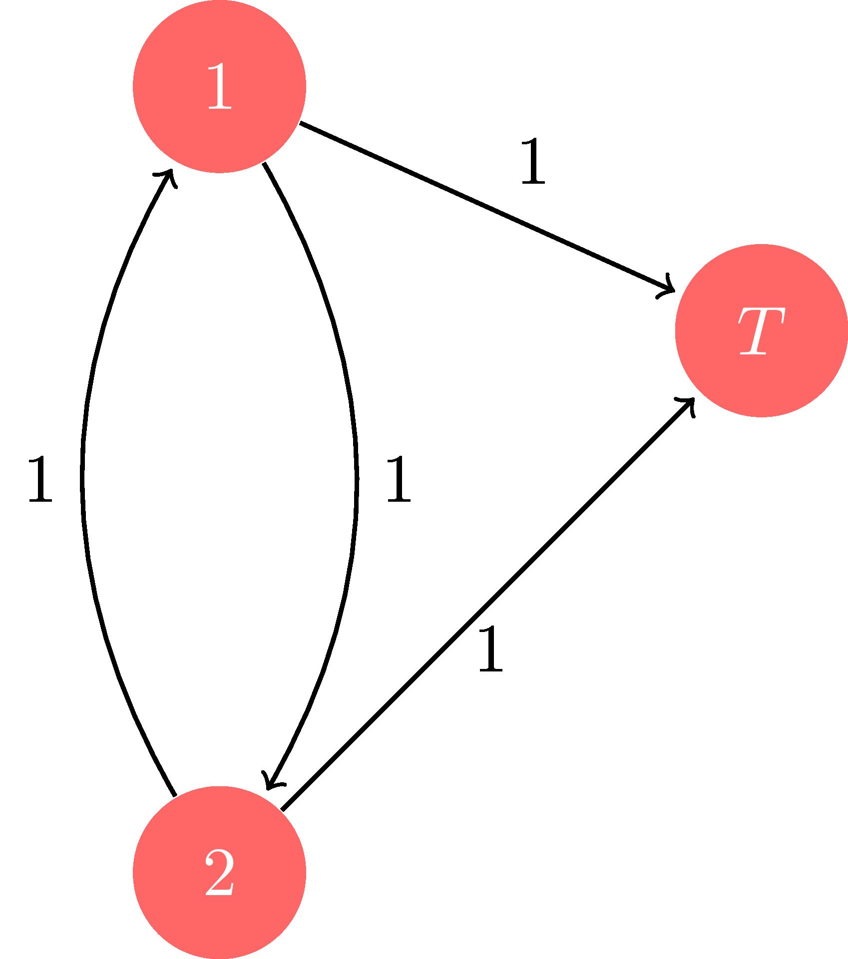
Figure 2.1: SSP example

It is obvious that the shortest path from node \(1\) (resp. \(2\)) to \(T\) follows the edge connecting it to \(T\), with a cost of \(1\). However, an improper policy is one that loops between \(1\) and \(2\). Since the edge costs are positive, it is clear that such an improper policy would incur infinite cost. On the other hand, having zero cost edges between \(1\) and \(2\) would mean the improper policy would incur zero cost in the long run – a pathological scenario that we would like to avoid. This discussion motivates the following assumptions:

(A1) There exists at least one proper policy.

(A2) For every improper policy \(\pi\), the associated cost \(J_\pi(i)\) is infinite for at least one state \(i\).

A sufficient condition for (A2) is \(\sum_{j=1}^n p_{ij}(a) g(i,a,j) > 0, i=1,\ldots,n, a\in A(i)\). For the sake of the discussion involving Bellman operators introduced below, one can assume that all policies are proper, i.e., each policy leads to the termination state with positive probability. The theory of SSP problem hold under a weaker condition where we include improper policies that have infinite cost.

We now claim that, under a proper policy, the probability of not reaching the termination state, from any given state, goes down to zero asymptotically. To see this, notice that for a proper policy \(\pi\), we have \[\begin{align} \mathbb{P}\left[i_{2n}\ne T \mid i_0=i,\pi\right] &= \mathbb{P}\left[i_{2n}\ne T \mid i_n\ne T,i_0=i,\pi\right] \mathbb{P}\left[i_{n}\ne T \mid i_0=i,\pi\right]\\ &\le \rho_\pi^2. \end{align}\] More generally, \[\mathbb{P}\left[i_{k}\ne T \mid i_0=i,\pi\right] \le \rho_\pi^{\lfloor\frac{k}{n}\rfloor}.\] Let \(g_k\) denote the cost incurred in the \(k\)th stage for a proper policy \(\pi\). Then, we have \[\mathbb{E}|g_k| \le \rho_\pi^{\lfloor\frac{k}{n}\rfloor} \max_{i=1,\ldots,n} | g(i,\pi(i)|,\] leading to \[|J_\pi(i)| \le \lim_{N\rightarrow\infty} \sum_{k=0}^{N-1} \rho_\pi^{\lfloor\frac{k}{n}\rfloor} \max_{i=1,\ldots,n} | g(i,\pi(i)| < \infty.\]

2.2 Bellman operators and fixed point relations

Recall that the state space \(\mathcal{X}= \{1,\ldots,n,T\}\) in a SSP problem. For any \(J = (J(1),\ldots,J(n))\), define the operator \(TJ=(TJ(1),\ldots,TJ(n))\) as follows: \[\begin{align} (TJ)(i) = \min_{a\in A(i)} \sum_{j\in\mathcal{X}} p_{ij}(a)\left(g(i,a,j)+J(j) \right), i=1,\ldots,n. \tag{2.2} \end{align}\] From the discussion of finite horizon problems, \(TJ\) can be interpreted as the optimal cost-to-go for an one stage problem with single stage cost \(g\) and terminal cost \(J\).

Further, we require another operator that is specific to a given policy \(\pi\). Define \(T_\pi\) as \[\begin{align} (T_\pi J)(i) = \sum_{j\in\mathcal{X}} p_{ij}(\pi(i))\left(g(i,\pi(i),j)+J(j) \right), i=1,\ldots,n. \end{align}\] Thus, \(T_\pi J\) is the cost-to-go for a given policy \(\pi\) in an one stage problem with single stage cost \(g\) and terminal cost \(J\).

We now introduce compact notation that simplifies the presentation of the results concerning the operators defined above. Let \[P^\pi=\begin{bmatrix} p_{11}(\pi(1)) & p_{12}(\pi(1)) & p_{13}(\pi(1)) & \dots & p_{1n}(\pi(1)) \\ p_{21}(\pi(2)) & p_{22}(\pi(2)) & p_{23}(\pi(2)) & \dots & p_{2n}(\pi(2)) \\ \vdots & \vdots & \vdots & \ddots & \vdots\\ p_{n1}(\pi(n)) & p_{n2}(\pi(n)) & p_{d3}(\pi(n)) & \dots & p_{nn}(\pi(n)) \end{bmatrix},\] and \(g_\pi = \left(g_\pi(1),\ldots,g_\pi(n)\right)\), where \(g_\pi(i) = \sum_{j\in\mathcal{X}} p_{ij}(\pi(i)) g(i,\pi(i),j)\). Then, it is easy to see that \[T_\pi J = g_\pi + P_\pi J.\] Let \((T^kJ)(i) = (T(T^{k-1}J))(i)\), \(i=1,\ldots,n\). Here \((T^0J)(i)=J(i).\ \forall i\). Similarly, let \((T_\pi^kJ)(i) = (T_\pi(T_\pi^{k-1}J))(i)\), \(i=1,\ldots,n\), with \((T_\pi^0J)(i)=J(i).\ \forall i\). As in the case of \(TJ\), \(T^kJ\) can be interpreted as the optimal cost-to-go for \(k\)-stage SSP with initial state \(i\), single stage cost \(g\) and terminal cost \(J\). Similarly, \(T_\pi^kJ\) can be interpreted as the cost-to-go of a stationary policy \(\pi\) for \(k\)-stage SSP with initial state \(i\), single stage cost \(g\) and terminal cost \(J\).

We now establish that the operators \(T\) and \(T_\pi\) are monotone.

Lemma 2.1 (Monotone Bellman operators) Suppose \(J,J'\) are two vectors in \(\mathbb{R}^n\) satisfying \(J(i) \le J'(i), \forall i\). Then, for any stationary \(\pi\), and for \(i=1,\ldots,n\), \(k=1,2,\ldots,\) we have

1. \((T^kJ)(i) \le (T^kJ')(i)\); and

2. \((T_\pi^kJ)(i) \le (T_\pi^kJ')(i)\).

Proof. Notice that \[\begin{align} (TJ)(i) &= \min_{a\in A(i)} \sum_{j\in\mathcal{X}} p_{ij}(a)\left(g(i,a,j)+J(j) \right)\\ & \le \min_{a\in A(i)} \sum_{j\in\mathcal{X}} p_{ij}(a)\left(g(i,a,j)+J'(j) \right) \end{align}\] The rest follows by induction and the second claim follows in a similar fashion. 

Lemma 2.2 (Constant shift lemma) Let \(\pi\) be a stationary policy, \(e\) a vector of ones, and \(\delta\) a positive scalar. Then, for \(i=1,\ldots,n\), \(k=1,2,\ldots,\) we have

1. \((T^k(J+\delta e))(i) \le (T^kJ)(i) + \delta\); and

2. \((T_\pi^k(J+\delta e))(i) \le (T_\pi^kJ)(i) + \delta\).

Further, the inequalities above are reversed for \(\delta < 0\).

Proof. Notice that \[\begin{align} (T(J+\delta e))(i) &= \min_{a\in A(i)} \sum_{j\in\mathcal{X}} p_{ij}(a)\left(g(i,a,j)+(J+\delta e)(j) \right)\\ &= \min_{a\in A(i)} \sum_{j\in\mathcal{X}} p_{ij}(a)\left(g(i,a,j)+J(j) + \delta \right)\\ &= \min_{a\in A(i)} \left[\sum_{j\in\mathcal{X}} p_{ij}(a)\left(g(i,a,j)+J(j)\right) + \sum_{j\in\mathcal{X}} p_{ij}(a)\delta \right]\\ &\le \min_{a\in A(i)} \left[\sum_{j\in\mathcal{X}} p_{ij}(a)\left(g(i,a,j)+J(j)\right) + \delta \right] \quad \textrm{(Since } \sum_{j\in\mathcal{X}} p_{ij}(a) \le 1)\\ &= \min_{a\in A(i)} \left[\sum_{j\in\mathcal{X}} p_{ij}(a)\left(g(i,a,j)+J(j)\right)\right] + \delta\\ & = (TJ)(i) + \delta. \end{align}\] The induction step follows by a compeletely parallel argument to the above, i.e., start with \(T^{k+1}\) on the LHS above and use \(T^k J\) in place of \(J\) on the RHS. The second claim follows in a similar fashion. 

Now, we establish a few important properties of the \(T_\pi\) operator in the proposition below.

Proposition 2.1 Assume (A1) and (A2). Then, we have

1. For any proper policy \(\pi\), the associated cost \(J_\pi\) satisfies \[\begin{align} \lim_{k\rightarrow \infty} (T_\pi^k J)(i) = J_\pi(i), \ i=1,\ldots,n,\tag{2.3} \end{align}\] for any \(J\). Further, \[J_\pi = T_\pi J_\pi,\] and \(J_\pi\) is the unique solution of the fixed point equation above.

2. A stationary policy \(\pi\) satisfying \[J(i) \ge (T_\pi J)(i), i=1,\ldots,n, \textrm{ for some } J, \textrm{ is proper.}\]

Proof. Recall that \[\begin{align} &T_\pi J = g_\pi + P_\pi J\\ \Rightarrow\quad & T_\pi^2 J = g_\pi + P_\pi T_\pi J = g_\pi + P_\pi g_\pi + P_\pi^2 J. \end{align}\] Proceeding similarly, we obtain \[\begin{align} T_\pi^j J = P_\pi^k J + \sum_{m=0}^{k-1} P_\pi^m g_\pi. \end{align}\] Since \(\pi\) is proper, we have \[\begin{align} \mathbb{P}\left[i_k \ne T \mid i_0=i,\pi\right] \le \rho_\pi^{\lfloor\frac{k}{n}\rfloor}, \textrm{ for } i=1,\ldots,n.(\#eq:inf1) \end{align}\] The condition above implies \[\lim_{k\rightarrow\infty} P_\pi^k J = 0.\] Thus, we have \[\lim_{k\rightarrow \infty} T_\pi^k J = \lim_{k\rightarrow \infty}\sum_{m=0}^{k-1} P_\pi^m g_\pi = J_\pi, \ i=1,\ldots,n,\] where the second limit exists from @ref\tag{2.4}.

Next, we prove that \(J_\pi\) is a fixed point of the operator \(T_\pi\). By definition, we have \[\begin{align} &T_\pi^{k+1} J = g_\pi + P_\pi T_\pi^k J \end{align}\] Taking limits as \(k\rightarrow \infty\) on both sides above and using @ref\tag{2.3}, we obtain \[\begin{align} &J = g_\pi + P_\pi J_\pi, \textrm{ or,} J_\pi = T_\pi J_\pi. \end{align}\] Next, to show that \(J_\pi\) is the unique fixed point, suppose that \(J\) satisfies \[J = T_\pi J.\] Then, \[T_\pi J = T_\pi^2 = J = \ldots\] leading to \[J = T_\pi^k J, \forall k\ge 1.\] Hence, \[J= \lim_{k\rightarrow \infty} T_\pi^k J = J_\pi.\] This proves the first claim.

For the second claim, let \(\pi\) be a stationary policy satisfying \(J\ge T_\pi J\) for some \(J\). Then, \(T_\pi J \ge T_\pi^2 J\) and so on, leading to \[J \ge T_\pi^k J = P_\pi^k J + \sum_{m=0}^{k-1} P_\pi^m g_\pi, \forall k\ge 1.\] If \(\pi\) is not proper, then \(J_\pi = \lim_{k\rightarrow\infty} \sum_{m=0}^{k-1} P_\pi^m g_\pi\) should diverge, and this leads to a contradiction since \(J(i) < \infty\) for each \(i\). Thus, \(\pi\) is proper, proving the second claim. 

We now turn our attention to the optimality operator \(T\) and prove a few important properties, which assist later in deriving dynamic programming based algorithms for solving SSPs.

Proposition 2.2 Assume (A1) and (A2). Let \(J^*(i) = \min_{\pi \in \Pi} J_\pi(i), i=1,\ldots,n\) denote the optimal cost and \(\pi^*\) be an optimal policy. Here \(\Pi\) denote the set of policies that satisfy (A1) and (A2). Then, we have

1. \(J^*\) satisfies \[J^* = T J^*.\] Moreover, \(J^*\) is the unique solution of the fixed point equation above.

2. For any \(J\), we have \[\begin{align} \lim_{k\rightarrow \infty} (T^k J)(i) = J^*(i), \ i=1,\ldots,n.(\#eq:tlim) \end{align}\]

3. A stationary policy \(\pi\) is optimal if and only if \[T_\pi J^* = T J^*.\]

Proof. We first show that \(T\) has at most one fixed point. Suppose \(J\) and \(J'\) are two fixed points of \(T\). Select policies \(\pi\) and \(\pi'\) such that \[\begin{align} J=TJ=T_\pi J, \textrm{ and } J'=TJ'=T_{\pi'} J'. \end{align}\] From the second claim in Proposition 1, we have \(\pi\) and \(\pi'\) are proper, and also that \(J=J_\pi\) and \(J'=J_{\pi'}\). Now, \[J = T^k J \le T^k_{\pi'} J, \forall k\ge 1,\] leading to \[J \le \lim_{k\rightarrow \infty} T_{\pi'}^k J = J_{\pi'} = J',\] where the first equality above follows from the first claim in Proposition 1.

Similarly, one can argue that \(J' \le J\) and hence, \(T\) has at most one fixed point.

Next, we show that \(T\) has at least one fixed point. Let \(\pi\) be a proper policy, whose existence is ensured by (A1). Let \(\pi'\) be another policy such that \[T_{\pi'} J_\pi = T J_\pi.\] Such a \(\pi'\) can be found from the set of finite policies in \(\Pi\).

Notice that \[J_\pi = T_\pi J_\pi \ge T J_\pi = T_{\pi'} J_\pi.\] Since \(J_\pi \ge T_{\pi'} J_\pi\), from the second claim in Proposition 1, we can infer that \(\pi'\) is proper. Further, \[T_{\pi'} J_\pi \ge T_{\pi'}^2 J_\pi \ge T_{\pi'}^3 J_\pi \ge \ldots\] implying \[J_\pi \ge \lim_{k\rightarrow\infty} T_{\pi'} J_\pi = J_{\pi'}.\] Continuing in this manner, we obtain a sequence of policies \(\{\pi_k\}\) such that each \(\pi_k\) is proper, and \[\begin{align} (\#eq:inf2) J_{\pi_k} \ge T J_{\pi_k} \ge J_{\pi_{k+1}}, \forall k \ge 1. \end{align}\] Since the set of policies is finite, some policy (say \(\pi\)) must be repeated in the sequence \(\{\pi_k\}\) and by @ref\tag{2.5}, we have \[J_\pi = T J_\pi.\] Thus, \(T\) has a fixed point and it is unique.

Next, we show that \(T^k J \rightarrow J_\pi\) as \(k\rightarrow \infty\) and later establish that \(J_\pi = J^*\).

Let \(e\) be a \(n\)-vector of ones and \(\delta >0\). Let \(\hat J\) be a vector satisfying \[T_\pi \hat J = \hat J - \delta e.\] Such a \(\hat J\) can be found, since we require \[\hat J = T_\pi \hat J + \delta e = g_\pi + \delta e + P_\pi \hat J,\] and \(\hat J\) corresponds to the cost of policy \(\pi\) with \(g_\pi\) replaced by \(g_\pi + \delta e\). Since \(\pi\) is proper, \(\hat J\) is unique (from Proposition 1). By construction, we have \[J_\pi \le \hat J, \textrm{ since } g_\pi \le g_\pi +\delta e.\] From the foregoing, we have \[J_\pi = T J_\pi \le T \hat J \le T_\pi \hat J = \hat J -\delta e \le \hat J,\] which implies \[J_\pi = T^k J_\pi \le T^k \hat J \le T^{k-1}\hat J \le \hat J, \forall k\ge 1.\] Thus, \(\{ T^k \hat J\}\) forms a bounded monotone sequence. Using monotone convergence theorem, we have \[\lim_{k\rightarrow \infty} T^k \hat J = \tilde J, \textrm{ for some } \tilde J.\] Applying \(T\) on both sides of the equation above, we obtain \[T\left(\lim_{k\rightarrow \infty} T^k \hat J\right) = T \tilde J.\] Since \(T\) is a continuous mapping, we can interchange the operator inside the limit to obtain \[T \tilde J = \lim_{k\rightarrow \infty} T^{k+1} \hat J = \tilde J.\] By uniqueness of the fixed point, we have \(\tilde J = J_\pi\), where \(\pi\) is the proper policy obtained earlier, while establishing the existence of fixed point of \(T\).

Now, we use a parallel argument to establish that \(\lim_{k\rightarrow \infty} T^{k} (J_\pi-\delta e) = J_\pi\). Notice that \[\begin{align} J_\pi - \delta e = T J_\pi - \delta e \le T(J_\pi - \delta e) \le T J_\pi =J_\pi,\tag{2.6} \end{align}\] where the last inequality follows from Lemma 2. From @ref\tag{2.6} and the fact that \(T(J_\pi - \delta e) \le T^2(J_\pi - \delta e)\le \ldots\), we have that \(\{T^k(J_\pi - \delta e)\}\) forms a monotonically increasing sequence that is bounded above, and hence convergent. As before, one can argue that \[\lim_{k\rightarrow \infty} T^{k} (J_\pi-\delta e) = J_\pi.\] Next, for any given \(J\), we can find a \(\delta > 0\) such that \[J_\pi -\delta e \le J \le \hat J.\] (Recall that \(\hat J\) corresponds to the cost of policy \(\pi\) with single stage cost \(g_\pi +\delta e\)). By monotonicity of \(T\) (see Lemma 1), we have \[T^k(J_\pi -\delta e) \le J \le T^k\hat J.\] Taking limits as \(k\rightarrow\infty\), and noting that both \(T^k(J_\pi -\delta e)\) and \(T^k \hat J\) converge to the same limit, i.e., \(J_\pi\), we have that \[\lim_{k\rightarrow\infty} T^k J = J_\pi.\]

To show that \(J_\pi = J^*\), take any policy \(\pi' = \{\mu_0,\mu_1,\ldots\}\). Then, \[T_{\mu_0}\ldots T_{\mu_{k-1}} \ge T^k J_0,\] where \(J_0\) is the \(n\)-vector of zeros. Taking limits as \(k\rightarrow\infty\) on both sides above, we have \[J_{\pi'} \ge J_\pi.\] Hence, \(\pi\) is the optimal policy and \(J_\pi = J^*\).

For proving the last part, suppose that \(\pi\) is optimal. Then \(J_\pi=J^*\), and by (A1) and (A2), \(\pi\) is proper. Using the first claim in Proposition 1, we obtain \[T_\pi J^* = T_\pi J_\pi = J_\pi = J^* = TJ^*.\] For the reverse implication, suppose that \(J^* = TJ^* = T_\pi J^*\). From the second claim in Proposition 1, we have that \(\pi\) is proper. Using the first claim in Proposition 1, we have \(J^* = J_\pi\), and hence, \(\pi\) is optimal. 

2.3 Examples

Example 2.1 (Time to termination) Consider a Stochastic Shortest Path problem where \[\begin{align} g(i, a) = 1 \textrm{,\: for } i=1\ldots n \end{align}\] The goal is to get to the terminal state as soon as possible. Let \(J^*(i)\) be the optimal expected cost when starting from state \(i\). By the Bellman equation we have \[\begin{align} J^*(i) = (TJ^*)(i)\textrm{, } \forall i \end{align}\] \[\begin{align} J^*(i) = \min_{a\in A(i)}[1+\sum_{j=1}^{n}P_{ij}(a)J^*(j)] \textrm{ , } \forall i \end{align}\] In the special case when there is only one action in each state, this model is equivalent to a Markov chain. In this case \(J^*(i)\) is the expected passage time to the terminal state \(T\). Let \(m_i\) denote this time instead of \(J^*(i)\). Then \[\begin{align} m_i = 1 + \sum_{j=1}^{n}P_{ij}m_j \textrm{ , for } i = 1 \ldots n \end{align}\] Solving the above system of equations yields \(m_i\), i.e. the expected passage time to the terminal state from each state \(i\).

Example 2.2 (The Spider and the Fly) A spider hunts a fly on the number line. The fly in each stage, jumps forward or backward \(1\) unit each with probability \(p\). It can remain in the same position with probability \(1 - 2p\) . The spider jumps towards the fly if the distance between them is greater than \(1\). If the distance between them is \(1\), the spider can choose to stay in its position hoping the fly will come to it or go \(1\) unit forward. The game (and the fly) ends when the spider is in the same position as the fly. The goal is to decide the actions of the spider so that the expected time to catch the fly is minimized.

SSP formulation : The problem can be formulated as an SSP with the state as the distance between the spider and the fly. The terminal state is state \(0\), which is when they are in the same position. Note that given an initial distance between the spider and the fly, the distance between them can only decrease. Therefore the states are finite. Assume that the spider and fly are initially at a separation of \(n\), then the state space \(S\) is \[\begin{align} S = \{ 0,1 \dots n \}. \end{align}\] The transition probabilities are obtained as follows: When the state is \(2\) or more, there is only one action for the spider, i.e. to jump towards the fly. The state will decrease by \(2\) if the fly jumps backward, it will decrease by \(1\) if it stays in its position and remain the same if the fly also jumps forward. Therefore, for \(i \geq 2\), \[\begin{align} &P_{i,i-2} = p, \ P_{i,i-1} = 1 - 2p, \textrm{ and } P_{i,i} = p. \end{align}\] = p.  \end{align} When the state is \(1\), there are \(2\) actions for the spider to take. Denote action "move" by \(M\) and "don’t move" by \(\overline{M}\). If the spider decides to move forward, then the distance will remain \(1\) if the fly moves either forward or backward. If the fly remains in the same position, then we go to terminal state \(0\). Therefore, \[\begin{align} &P_{1,1}(M) = 2p, \quad P_{1,0}(M) = 1 - 2p. \end{align}\] If the spider decides to stay in its position, then the distance (and hence the state) will increase to \(2\) if the fly moves forward, it will remain \(1\) if the fly does not move and becomes \(0\) if the fly moves backward. Therefore, \[\begin{align} P_{1,2}(\overline{M}) = p, P_{1,0}(\overline{M}) = p, \textrm{ and } P_{1,1}(\overline{M}) = 1 -2p. \end{align}\] As we want to find the minimum expected time to catch the fly, we can set all the single state costs to \(1\) so that the expected cost is a measure of how quickly the spider meets the fly.

The Bellman Equation: As there is only one action to take for states \(i>1\), the Bellman equation for \(i>1\) is \[\begin{align} J^*(i) &= \sum_{j=1}^n P_{i,j}\left( g(i,a,j) +J^*(j)\right)\\ & = P_{i,i-2}\left(1+ J^*(i-2)\right) + P_{i,i-1}\left(1+ J^*(i-1)\right) + P_{i,i}\left( 1+ J^*(i)\right)\\ & = p\left( 1+ J^*(i-2)\right) + (1-2p)\left(1+ J^*(i-1)\right) + p\left(1+ J^*(i)\right)\\ & = 1 + p J^*(i-2) + (1-2p)J^*(i-1)+ p J^*(i). \end{align}\] On the other hand, for state \(1\), we have to take the minimum over the two admissible actions as follows: \[\begin{align} J^*(1) &= \min \left(\sum_{j=1}^n P_{1,j}\left( g(1,M,j) +J^*(j)\right),\: \sum_{j=1}^n P_{1,j}\left( g(1,\overline{M},j) +J^*(j)\right) \right)\\ &= \min \left(1+2pJ^*(1)+(1-2p)J^*(0),\:1+pJ^*(2)+pJ^*(0)+(1-2p)J^*(1) \right)\\ &= 1+ \min \left(2pJ^*(1),\: pJ^*(2)+(1-2p)J^*(1) \right). \end{align}\] Also, as \(0\) is the terminal state, we have \(J^*(0) = 0\). Hence, we obtain \[\begin{align} J^*(i) = \begin{cases} 1 + pJ^*(i-2) + (1-2p)J^*(i-1) + pJ^*(i) & \textrm{when} \: i \geq 2\\ 1 + \min(2pJ^*(1), \:pJ^*(2) + (1-2p)J^*(1)) & \textrm{when} \: i = 1\\ 0 & \textrm{when} \: i = 0 \tag{2.7} \end{cases} \end{align}\] Substituting \(i = 2\) in (2.7), we obtain \[\begin{align} J^*(2) &= 1 + pJ^*(0) + (1-2p)J^*(1) + pJ^*(2)\\ \implies J^*(2) &= \frac{1}{1-p} + \frac{(1-2p)J^*(1)}{1-p}. \tag{2.8} \end{align}\] Using (2.8) in (2.7), we obtain \[\begin{align} J^*(1) &= 1 + \min\left[ 2p J^*(1), \: \frac{p}{1-p}+\frac{p(1-2p)J^*(1)}{1-p} + (1-2p)J^*(1)\right]\\ \implies J^*(1) &= 1 + \min \left [ 2p J^*(1), \: \frac{p}{1-p} + \frac{(1-2p)J^*(1)}{1-p} \right]. \end{align}\] Let the first term in the minimum be \(A\) and the second term \(B\). This gives us the following two cases:

1. Case \(A > B\) \[\begin{align} J^*(1) = 1 + \frac{p}{1-p} + \frac{(1-2p)J^*(1)}{1-p} \implies J^*(1) = \frac{1}{p} \end{align}\] under the condition \[\begin{align} 2p J^*(1) &> \frac{p}{1-p} + \frac{(1-2p)J^*(1)}{1-p}\\ \implies 2 &> \frac{p}{1-p} + \frac{(1-2p)}{p(1-p)}\\ \implies 2 &> \frac{(1-p)^2}{p(1-p)}\\ \implies p &> 1/3 \end{align}\] In this case, the optimal action is \(\overline{M}\) i.e. to not move.

2. Case \(A < B\) \[\begin{align} J^*(1) = 1 + 2pJ^*(1) \implies J^*(1) = \frac{1}{1-2p}. \end{align}\] The optimal action is \(M\), i.e., to jump towards the fly, under the following condition: \[\begin{align} 2p J^*(1) &\leq \frac{p}{1-p} + \frac{(1-2p)J^*(1)}{1-p}\\ \textrm{ or, equivalently, } \frac{2p}{1-2p} &\leq \frac{1+p}{1-p}\\ \textrm{ or, equivalently, } \frac{1}{1-2p} &\leq \frac{2}{1-p}\\ \textrm{ or, equivalently, } p \leq \frac{1}{3} \end{align}\]

Therefore, the optimal policy is \[\begin{align} \pi_{i} = \begin{cases} M &\textrm{when $i = 1$ and $p \leq \frac{1}{3}$},\\ \overline{M} &\textrm{when $i = 1$ and $p > \frac{1}{3}$}\\ \textrm{don't care} &\textrm{when $i \geq 2$} \end{cases} \end{align}\] and the corresponding expected costs are given by \[\begin{align} J^*(i) = \begin{cases} 0 &\textrm{when $i = 0$}\\ \frac{1}{1 - 2p} &\textrm{when $i = 1$ and $p \leq \frac{1}{3}$}\\ \frac{1}{p} &\textrm{when $i = 1$ and $p > \frac{1}{3}$}\\ 1 + pJ^*(i-2) + (1-2p)J^*(i-1) + pJ^*(i) &\textrm{when $i \geq 2$.} \end{cases} \end{align}\]

2.4 Bellman operator in SSPs: The contractive case

Proposition 2.3 Assume that all policies are proper. Then,

1. The Bellman optimalty operator \(T\) is a contraction with respect to a weighted max-norm. In other words, there exists a vector \(\xi = \{\xi(1), ..., \xi(n)\}\) such that \(\xi(i) > 0 \ \forall i = 1,...n\) and a scalar \(0 < \rho < 1\) such that \[\begin{align} \left\Vert T J - T \bar{J} \right\Vert_{\xi} \leq \rho \cdot \left\Vert J - \bar{J} \right\Vert_{\xi} \ \forall J, \bar{J} \in \mathbb{R}^n \end{align}\] where \[\begin{align} \left\Vert J \right\Vert_{\xi} = \max_{i=1,...n} \frac {|J(i)|} {\xi(i)} \end{align}\]

2. For a stationary policy \(\pi\), Bellman optimalty operator \(T_{\pi}\) is a contraction with respect to a weighted max-norm. In other words, there exists a vector \(\xi = \{\xi(1), ..., \xi(n)\}\) such that \(\xi(i) > 0 \ \forall i = 1,...n\) and a scalar \(0 < \rho < 1\) such that \[\begin{align} \left\Vert T_{\pi} J - T_{\pi} \bar{J} \right\Vert_{\xi} \leq \rho \cdot \left\Vert J - \bar{J} \right\Vert_{\xi} \ \forall J, \bar{J} \in \mathbb{R}^n \end{align}\] where \[\begin{align} \left\Vert J \right\Vert_{\xi} = \max_{i=1,...n} \frac {|J(i)|} {\xi(i)} \end{align}\]

Proof. Let us create the vector \(\xi\) that satisifies the proposition. Consider a new SSP where transition probabilities are same as in the original, but the transition cost are all equal to \(-1\) except at the self-transition in the terminal states whose cost is still \(0\). So, \[\begin{align} g(i, a, j) = \begin{cases} 0 \quad i = j = T \land \forall a \in A(T)\\ -1 \quad else \end{cases} \end{align}\] Let \(\hat{J}\) be the optimal cost of this new SSP. Using Bellman equation, we get \[\begin{align} \hat{J}(i) &= -1 + \min_{a \in A(i)} \Sigma_{j=1}^{n} p_{ij}(a) \hat{J}(j)\\ &= T \hat{J}(i)\\ &\leq T_{\pi} \hat{J}(i) \ \textit{(For any proper policy $\pi$)}\\ &\leq -1 + \Sigma_{j=1}^{n} p_{ij}(\pi(i)) \hat{J}(j) \end{align}\] Let \(\xi = -\hat{J}\). Since all costs in the new SSP are non-positive and since every policy must take atleast one transition to reach the termination state, \(\hat{J}(i)\) is less than \(-1\) for all \(i = 1,..., n\). Hence \(\xi(i) \geq 1\) for all \(i = 1,..., n\) For all proper policy, we have \[\begin{align} & - \hat{J}(i) \ge 1 + \Sigma_{j=1}^{n} p_{ij}(\pi(i)) (- \hat{J}(j)) \ \textit{Or, equivalently,}\\ & \xi(i) \ge 1 + \Sigma_{j=1}^{n} p_{ij}(\pi(i)) \xi(j). \end{align}\] \[\begin{align} \Sigma_{j=1}^{n} p_{ij}(\pi(i)) \xi(j) \le \xi(i) - 1 \le \rho \cdot \xi(i), \tag{2.9} \end{align}\] where \[\begin{align} \rho = \max_{i=1,... n} \frac {\xi(i) - 1} {\xi(i)} < 1 \end{align}\] Now, for any proper policy \(\pi\) and \(J, \bar{J}\), \[\begin{align} |T_{\pi} J(i) - T_{\pi} \bar{J}(i)| &= | \Sigma_{j=1}^{n} p_{ij}(\pi(i))(J(j) - \bar{J}(j)) |\\ &\leq \Sigma_{j=1}^{n} p_{ij}(\pi(i)) | J(j) - \bar{J}(j) |\\ &\leq \Sigma_{j=1}^{n} p_{ij}(\pi(i))\xi(j) | \frac {J(j) - \bar{J}(j)} {\xi(j)} |\\ &\leq (\Sigma_{j=1}^{n} p_{ij}(\pi(i))\xi(j)) \cdot (\max_{j=1,...n} | \frac {J(j) - \bar{J}(j)} {\xi(j)} |)\\ &\leq \rho \cdot \xi(i) \cdot (\max_{j=1,...n} | \frac {J(j) - \bar{J}(j)} {\xi(j)} |) \tag{2.10} \\ | \frac{T_{\pi} J(i) - T_{\pi} \bar{J}(i)} {\xi(i)} | &\leq \rho \cdot (\max_{j=1,...n} | \frac {J(j) - \bar{J}(j)} {\xi(j)} |)\\ \max_{i=1,...n} | \frac{T_{\pi} J(i) - T_{\pi} \bar{J}(i)} {\xi(i)} | &\leq \rho \cdot (\max_{j=1,...n} | \frac {J(j) - \bar{J}(j)} {\xi(j)} |)\\ \left\Vert T_{\pi} J - T_{\pi} \bar{J} \right\Vert_{\xi} &\leq \rho \cdot \left\Vert J - \bar{J} \right\Vert_{\xi}, \end{align}\] where we used (2.9) in arriving at (2.10).

So \(T_{\pi}\) is a contraction with respect to \(\left\Vert \cdot \right\Vert_{\xi}\) with modulus \(\rho\). Hence, the second claim in the proposition statement follows.

We have shown already that \[\begin{align} |T_{\pi} J(i) - T_{\pi} \bar{J}(i)| \leq \rho \cdot \xi(i) \cdot \left\Vert J - \bar{J} \right\Vert_{\xi}\\ \end{align}\] Now consider two cases: \(T_{\pi} J(i) > T_{\pi} \bar{J}(i)\) and \(T_{\pi} \bar{J}(i) \le T_{\pi} \bar{J}(i)\). For case \(1\), \[\begin{align} T_{\pi} J(i) &\leq T_{\pi} \bar{J}(i) + \rho \cdot \xi(i) \cdot \left\Vert J - \bar{J} \right\Vert_{\xi}\\ \end{align}\] Taking minimum over \(\pi\) on both sides to obtain \[\begin{align} T J(i) &\leq T \bar{J}(i) + \rho \cdot \xi(i) \cdot \left\Vert J - \bar{J} \right\Vert_{\xi}\\ T J(i) - T \bar{J}(i) &\leq \rho \cdot \xi(i) \cdot \left\Vert J - \bar{J} \right\Vert_{\xi}\\ |T J(i) - T \bar{J}(i)| &\leq \rho \cdot \xi(i) \cdot \left\Vert J - \bar{J} \right\Vert_{\xi}\\ \frac {|T J(i) - T \bar{J}(i)|} {\xi(i)} &\leq \rho \cdot \left\Vert J - \bar{J} \right\Vert_{\xi}\\ \max_{i=1,...n} \frac {|T J(i) - T \bar{J}(i)|} {\xi(i)} &\leq \rho \cdot \left\Vert J - \bar{J} \right\Vert_{\xi}\\ \left\Vert T J - T \bar{J} \right\Vert_{\xi} &\leq \rho \cdot \left\Vert J - \bar{J} \right\Vert_{\xi}\\ \end{align}\] Similarly case \(2\) can also be made to yield the same result.

Hence, \(T\) is also a contraction with respect to \(\left\Vert \cdot \right\Vert_{\xi}\) with modulus \(\rho\). The first claim in the proposition statement follows.  

2.5 Contraction mappings: An introduction

Consider the function \(f(x) = \frac {x} {2}\). This function has a unique fixed point which is \(0\) i.e. \(f(x) = x \implies x=0\). Also for any \(x\), \(\lim_{n\to\infty} f^n(x) = \lim_{n\to\infty} \frac {x} {2^n} = 0\). So we will get the fixed point of the function by repeatedly applying \(f\) on any value. Also everytime we apply \(f\), we get nearer to the fixed point on a geometric rate. For e.g., on initial value \(16\), we get exponentially closer to \(0\) with each application of \(f\) as \(8, 4, 2, 1, 0.5, ...\)

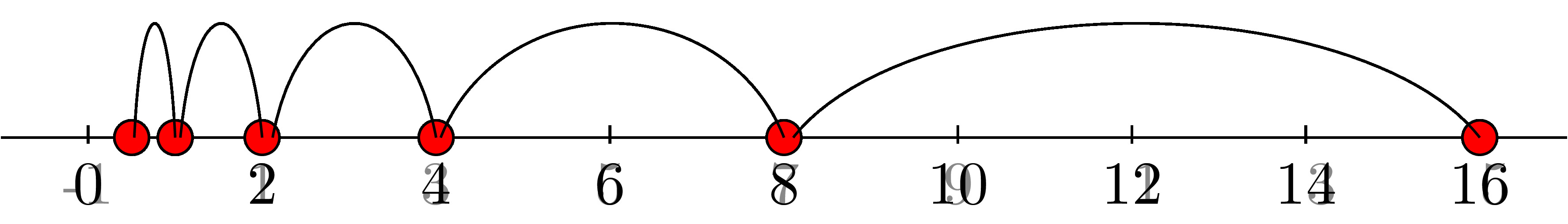
Figure 2.2: Illustration of the contraction principle

A norm on Vector space \(\mathcal{X}\) is a function \(\left\Vert \cdot \right\Vert:\mathcal{X} \to \mathbb{R}\) with the following properties:

1. \(\left\Vert x \right\Vert = 0\) iff \(x=0\)

2. \(\left\Vert x+y \right\Vert \le \left\Vert x \right\Vert + \left\Vert y \right\Vert,\ \forall x,y \in \mathcal{X}\)

3. \(\left\Vert cx \right\Vert = |c| \cdot \left\Vert x \right\Vert,\ \forall x \in \mathcal{X}, c \in \mathbb{R}\)

A function \(F:\mathcal{X}\to \mathcal{X}\) is a contraction mapping if for some \(\rho \in (0, 1)\), \[\left\Vert F(x) - F(y) \right\Vert \leq \rho \cdot \left\Vert x - y \right\Vert, \forall x,y \in \mathcal{X}\\\] The scalar \(\rho\) is called the modulus of contraction of \(F\).

The space \(\mathcal{X}\) is complete under the norm \(\left\Vert \cdot \right\Vert\) if every Cauchy sequence \(\{x_k\} \subset \mathcal{X}\) converges. A sequence \(\{x_k\}\) is Cauchy if for any \(\epsilon > 0\) there exists some \(N\) such that \(\left\Vert x_m - x_n \right\Vert \le \epsilon,\ \forall m,n \ge N\).

Let \(F:\mathcal{X}\to \mathcal{X}\) be a contraction mapping such that \(\mathcal{X}\) is conmplete under the norm \(\left\Vert \cdot \right\Vert\). Then two important properties hold:

1. \(F\) has a unique fixed point (i.e) \(\exists x^*, F(x^*) = x^*\).

2. The sequence \(\{x_k\}\) generated by the iteration \(x_{k+1} = F(x_k)\) converges to \(x^*\) for any initial point \(x_0\).

These two properties will be proved in a specialized setting in the next subsection. But these properties hold in the general case as well.

We now discuss contraction mappings in the context of MDPs. The result below shows that a contraction mapping has a fixed point, and repeated application of the mapping leads to this fixed point.

Theorem 2.1 (Fixed point theorem) Let \(B(\mathcal{X})\) denote all functions \(J\) such that \(\left\Vert J \right\Vert_{\xi} < \infty\) . Let \(F:B(\mathcal{X})\to B(\mathcal{X})\) be a contraction mapping with \(\rho\) \(\in (0,1)\). Assuming \(B(\mathcal{X})\) is complete, we have,

1. There exists a unique \(J^*\) \(\in B(\mathcal{X})\) such that \[\begin{align} J^* = FJ^* \end{align}\]

2. The value iteration converges \[\begin{align} \lim_{k\rightarrow\infty} F^k J_0 = J^* \end{align}\]

3. The value iteration error is bounded \[\begin{align} \left\Vert F^k J_0 - J^* \right\Vert_{\xi} \leq \rho^k \cdot \left\Vert J_0 - J^*\right\Vert_{\xi} \end{align}\]

:::

Proof. Let us fix some \(J_0\) \(\in B(\mathcal{X})\). Now we set \(J_{k+1} = F J_k\) starting with \(J_0\). Since \(F\) is a contraction mapping, we have, \[\left\Vert J_{k+1} - J_k\right\Vert_{\xi}\ \leq \rho \cdot \left\Vert J_{k} - J_{k-1}\right\Vert_{\xi}\] Applying the same inequality, we end up getting, \[\left\Vert J_{k+1} - J_k\right\Vert_{\xi} \leq \rho^k \cdot \left\Vert J_{1} - J_{0}\right\Vert_{\xi} \tag{*}\] So, \(\forall k \geq 0 , \forall m \geq 1\), we get \[\left\Vert J_{k+m} - J_{k}\right\Vert_{\xi} = \left\Vert (J_{k+m} - J_{k+m-1}) + (J_{k+m-1} - J_{k+m-2}) + \dots + (J_{k+1} - J_k)\right\Vert_{\xi}\] Using triangular inequality, we get, \[\left\Vert J_{k+m} - J_{k}\right\Vert_{\xi} \leq \sum_{i=1}^{m} \left\Vert J_{k+i} - J_{k+i-1}\right\Vert_{\xi}\] Substituting the equation \((*)\) we get, \[\left\Vert J_{k+m} - J_{k}\right\Vert_{\xi} \leq \rho^k (1 + \rho + \dots + \rho^{m-1}) \left\Vert J_1-J_0\right\Vert_{\xi}\] Since \(\rho < 1\), \((1 + \rho + \dots +\rho^{m-1}) < \frac{1}{1-\rho}\). Hence, we get, \[\left\Vert J_{k+m} - J_{k}\right\Vert_{\xi} \leq \frac{\rho^{k}}{1-\rho}\left\Vert J_1-J_0\right\Vert_{\xi}\] Hence, \(\{J_k\}\) forms a Cauchy sequence. Since \(B(\mathcal{X})\) is complete, \(J_k \to J^*\), and \(J^* \in B(\mathcal{X})\) Now, given this background, we can show that \(J^*\) is a fixed point of the contraction mapping \(F\) . Using the triangular inequality, we have, \[\left\Vert F J^* - J^*\right\Vert_{\xi}\ \leq \left\Vert F J^* - J_{k}\right\Vert_{\xi} + \left\Vert J_{k} - J^*\right\Vert_{\xi}\] Since F is a contraction mapping, and \(J_k = F J_{k-1}\), we get, \[\left\Vert F J^* - J^*\right\Vert_{\xi}\ \leq \rho \left\Vert J^*- J_{k-1}\right\Vert_{\xi} + \left\Vert J_{k} - J^*\right\Vert_{\xi}\] As \(k \to \infty, J_{k} \to J^*\), and the RHS tends to 0. As a result, \[\left\Vert F J^* - J^*\right\Vert_{\xi}\ \leq 0\] So, \(F J^* = J^*\). That is, \(J^*\) is a fixed point for the contraction mapping \(F\). Now, we show that \(J^*\) is unique. Assume \(\tilde{J}\) is another fixed point, that is, \(F \tilde{J} = \tilde{J}\) \[\left\Vert J^* - \tilde{J} \right\Vert_{\xi} = \left\Vert F J^* - F\tilde{J} \right\Vert_{\xi}\] Since F is a contraction mapping, we get \[ \left\Vert J^* - \tilde{J} \right\Vert_{\xi} \leq \rho \left\Vert J^* - \tilde{J} \right\Vert_{\xi}\] Since \(\rho < 1\), this is only possible if \(\left\Vert J^* - \tilde{J} \right\Vert_{\xi} = 0\). That is, \(\tilde{J} = J^*\). We now show that the value iteration error is bounded. \[\begin{align} \left\Vert F^k J_0 - J^* \right\Vert_{\xi} &= \left\Vert F^k J_0 - F J^* \right\Vert_{\xi}\\ & \leq \rho \left\Vert F^{k-1} J_0 - J^* \right\Vert_{\xi}\\ & \leq \rho^2 \left\Vert F^{k-2} J_0 - J^* \right\Vert_{\xi}\\ &\vdots\\ & \leq \rho^k \left\Vert J_0 - J^* \right\Vert_{\xi}\\ \end{align}\] That is, the error in the \(k^{th}\) iteration is bounded by \(\rho^k \left\Vert J_0 - J^* \right\Vert_{\xi}\) 

Returning to the stochastic shortest path problem, we can apply the theorem to get an error bound. Assuming all policies are proper, \(\exists\) \(\xi\) such that \(\xi(i)>0\) \(\forall\) \(i\) and \[\begin{align} \left\Vert TJ - T\overline{J} \right\Vert_{\xi} \leq \rho \left\Vert J - \overline{J} \right\Vert_{\xi} , \forall J, \overline{J} \in \mathbb{R}^n \end{align}\]

2.6 Value iteration

2.6.1 Basic algorithm

1. Initialize \(J\) with any value \(J_0\).

2. Repeatedly update \(J\) by applying \(T\) over it such that \(J_{k+1} = T J_k\).

This will result in \(T^*\) since we know that \(\lim_{k\rightarrow\infty} T^k J_0 = J^*\) for any \(J_0\).

Using the error bound we proved as the second claim in proposition 4, we can simplify the equation to \[\begin{align} \left\Vert J_k - J^* \right\Vert_{\xi} \leq \rho^k \left\Vert J_0 -J^* \right\Vert_{\xi}\end{align}\] where \(J_i = TJ_{i-1}\) \(\forall \; i\) and \(J_0\) is the initial vector for value iteration. Remarks:

1. A similar error bound holds for evaluation a proper policy \(\pi\) using value iteration.

2. For the proof of contraction mapping we require that all policies be proper.

2.6.2 Gauss-Seidel value iteration

In regular value iteration, when we calculate \(J_k = TJ_{k-1}\), we apply the operator for all states i together. Alternatively, we could update 1 state at a time and use the most recent updates of each state. This is the idea behind the Gauss-Seidel Variant.

The update rule of Gauss Seidel variant is as follows: For the \(1^{st}\) state, \[\begin{align} (FJ) (1) = \min_{a \in A(1)} \sum_j p_{1j}(a)(g(1,a,j) +J(j)) \end{align}\]

which is the same as (TJ)(1) For \(i^{th}\) state, \(i = 2,\dots,n\) \[\begin{align} (FJ) (i) = \min_{a \in A(i)} \sum_j p_{ij}(a)(g(i,a,j)) +\sum_{j=1}^{i-1} p_{ij}(a)(FJ)(j)+\sum_{j=i}^{n} p_{ij}(a) J(j) \end{align}\]

Remark: It can be shown that the Gauss-Seidel variant of value iteration converges to \(J^*\) and that it does so faster than regular value iteration. (Section 2.2 of (D. P. Bertsekas 2012)) More precisely, \[\begin{align} \left\Vert J^{VI}_k - J^* \right\Vert_{\xi} \geq \left\Vert J^{GSVI}_k - J^* \right\Vert_{\xi}\end{align}\]

2.6.3 Asynchronous value iteration

The algorithm for asynchronous value iteration is as follows

1. Start with an arbitrary \(J_0\)

2. In the \(k^{th}\) iteration, pick an index \(i_k \in\{1,2,\dots n \}\) and calculate \[\begin{align} J_{k+1}(i) = \begin{cases} (TJ_k)(i) & \:if \;i=i_k\\ J_k(i) & \: else \end{cases} \end{align}\]

Assuming all the states \(\{1,2,\dots,n\}\) are picked infinitely often, it can be proved that \[\begin{align} J_k \to J^* \: as \: k \to \infty \end{align}\]

2.6.4 Q-Factors and Q-Learning

Q factors underly the popular Q-learning algorithm. In a typical RL setting, to be introducted in later chapter, the transition probabilities are not known and hence, the Bellman equation cannot be solved directly or via value iteration. In such settings, Q-factors are useful in implementing a value iteration type algorithm albeit with sample trajectories. We first present a version of Q-learning, where the MDP model is known and in this case, the Q-learning algorithm is a special case of value iteration.

In an SSP, the value iteration update is: \(J_{k+1} = T J_k\) Expanding that for each state, \[J_{k+1}(i) = \min_{a \in \mathcal{A}(i)} \sum_{j \in \mathcal{X}} p_{ij}(a) (g(i,a,j) + J_k(j)) \qquad \qquad i=1,\ldots,n.\] We can rewrite this as \[\begin{align} J_{k+1}(i)= \min_{a \in \mathcal{A}(i)} Q_{k+1}(i,a) \qquad \qquad i=1,\ldots,n , \forall a \in \mathcal{A}(i),\tag{2.11} \end{align}\] where \[\begin{align} Q_{k+1}(i,a) &= \sum_{j \in \mathcal{X}} p_{ij}(a) (g(i,a,j) + J_k(j)) (\#eq:Qfactoreqn2)\\ &= \sum_{j \in \mathcal{X}} p_{ij}(a) (g(i,a,j) + \min_{b \in \mathcal{A}(j)} Q_{k}(j,b)) \ i=1,\ldots,n , \forall a \in \mathcal{A}(i)(\#eq:Qfactoreqn3) \end{align}\] So far we have just manipulated the value iteration equation to introduce a new variable Q. In particular, @ref\tag{2.12} is obtained from @ref\tag{2.13} by using @ref\tag{2.11}. These three equations form the Q-learning update.

Just as we defined \(J^{*}\) after defining \(J\), we can analogously define \(Q^{*}\) as follows: \[\begin{align} Q^{*}(i,a) = \sum_{j \in \mathcal{X}}p_{ij}(a)(g(i,a,j) + J^{*}(j)) \qquad \qquad i=1,\ldots,n , \forall a \in \mathcal{A}(i). \end{align}\] While \(J^{*}(i)\) represents the optimal cost starting from state \(i\), \(Q^*(i,a)\) represents the optimal cost when you start at state \(i\) and the first action from there is action \(a\). In other words, taking action \(a\) in state \(i\) and following the optimal policy thereafter leads to a total cost of \(Q^*(i,a)\). The terms \(Q^{*}(i,a)\) are called Q-factors or Q-values.

From the Bellman equation \(J^{*} = TJ^{*}\) we have, \[\begin{align}(\#eq:Qstar_eqn1) J^{*}(i) = \min_{a \in \mathcal{A}(i)} Q^{*}(i,a) \qquad \qquad i = 1,2 \cdots n \end{align}\] Then \(Q*\) can be alternatively defined as : \[\begin{align} Q^{*}(i,a) &= \sum_{j \in \mathcal{X}} p_{ij}(a)(g(i,a,j) + J^{*}(j)) (\#eq:Qstar_eqn2)\\ \implies Q^{*}(i,a) &= \sum_{j \in \mathcal{X}} p_{ij}(a)(g(i,a,j) + \min_{b \in \mathcal{A}(j)} Q^{*}(j,b)) \qquad \qquad i=1,\ldots,n , \forall a \in \mathcal{A}(i) (\#eq:QBellman_eqn)\end{align}\] Again, Eqn @ref(#eq:QBellman_eqn) was obtained by substituting Eqn @ref(#eq:Qstar_eqn1) appropriately in Eqn @ref(#eq:Qstar_eqn2) Eqn @ref(#eq:QBellman_eqn) forms a system of equations (when iterated over all valid \((i,a)\)) for \(Q^{*}\) called the Q-Bellman Equation, just as the Bellman Equation was a system of equations for \(J^{*}\). Just as we used the Bellman Optimality Operator to represent the Bellman Equation, the operator underlying the Q-Bellman Equation is \[(FQ)(i,a) = \sum_{j \in \mathcal{X}} p_{ij}(a)(g(i,a,j) + \min_{a \in \mathcal{A}(j)}Q(j,b)) \qquad \qquad i=1,\ldots,n , \forall a \in \mathcal{A}(i)\] Operator \(F\) takes some \(Q\) and gives \(FQ\) according to the above equation. The difference between this and the operator \(T\) (Eqn @ref\tag{2.2}) is that the \(\min\) is at the end of the equation, instead of being at the beginning. This is because action \(a\) is fixed, and we have to optimize further actions only later on after we reach state \(j\). The equations for \(Q\) and \(Q^{*}\) are just re-arranged versions of the equations for \(J,J^{*}\) when \(p_{ij}\)’s are known. When the model is not known we have to use approximate estimates for \(J\) and \(Q\). The Bellman and Q-Bellman Equations then (very loosely stated) look like expectations of some variable. However in the Bellman Equation the \(\min\) is outside the expectation , making it hard to estimate, while it is much easier to do in the Q-Bellman equation where the \(\min\) is far inside the equation (Loosely speaking, it is easy to estimate an expectation, but not the minimum of some expectation). Even though Q-learning is useful when the model is not known, even in the model based setting Bertsekas uses the notation ‘Q-learning’. So Value Iteration for Q-Bellman equation is as follows. Start with some \(Q_0\) and keep applying \(F\) operator. Eventually \(Q*\) will be obtained. \[Q_0 \xrightarrow{\text{F}} Q_1 \xrightarrow{\text{F}}Q_2 \cdots \xrightarrow{\text{F}} Q^{*}\] \[Q_{k+1} = FQ_k\] \[\lim_{k \to \infty} Q_k = Q^{*}\] From \(Q^{*}\) , \(J^{*}\) can be found using Eqn @ref(#eq:Qstar_eqn1).

2.7 Policy iteration

Value iteration can possibly take infinite number of steps to converge. Policy iteration, on the other hand, is "guaranteed" to converge within a finite number of iterations.

Policy Iteration can be broken down to into two steps that are conducted one after the other; policy evaluation and policy improvement. The two steps continue in a cycle till the optimal policy is found.

The algorithm starts with \(\pi_0\) and iterates as long as \[\begin{align} J_{\pi_0} \geq J_{\pi_1} \dots\end{align}\] This inequality, after each iteration has to be strict for atleast 1 state. If not (i.e, if \(J_{\pi_k} = J_{\pi_{k+1}}\)), then we have found the optimal policy.

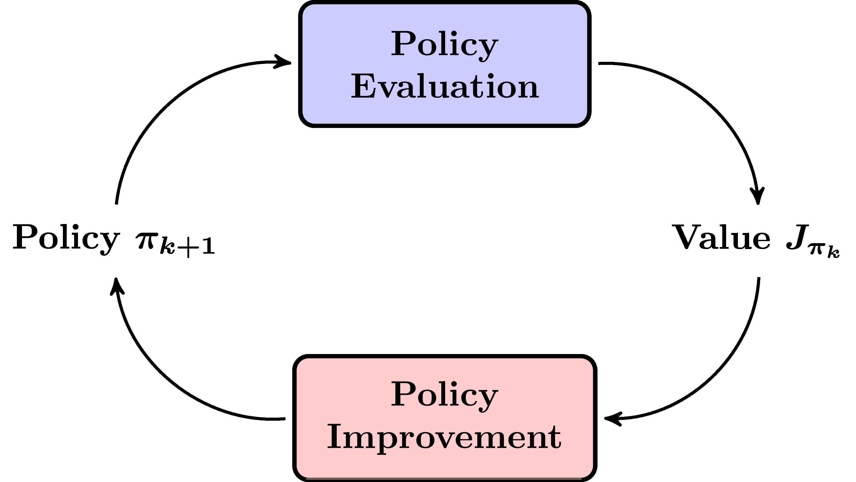
Figure 2.3: Policy iteration

2.7.1 Basic algorithm

1. Start with \(k = 0\) and a proper policy \(\pi_k\)

2. Policy Evaluation : Evaluate \(\pi_k\), i.e., compute \(J_{\pi_k}\) by solving \[J_{\pi_k} = T_{\pi_k} J_{\pi_k}\] \[\implies J_{\pi_k} = \sum_{j \in \mathcal{X}} p_{ij}(\pi_k(i))(g(i,\pi_k(i),j) + J_{\pi_k}(j)) \qquad \qquad i = 1 \cdots n\] Here \(J_{\pi_1},J_{\pi_2} \cdots J_{\pi_n}\) are unknowns that can be found by the above set of equations.

3. Policy Improvement : Find a new policy using \[T_{\pi_{k+1}} J_{\pi_k} = T J_{\pi_k}\] \[\implies \pi_{k+1}(i) = \mathop{\textrm{ arg\,min}}_{a \in \mathcal{A}(i)} \sum_{j in \mathcal{X}} p_{ij}(a)(g(i,a,j) + J_{\pi_k}(j)) \qquad \qquad i = 1 \cdots n\] If \(J_{\pi_{k+1}}(i) < j_{\pi_k}(i)\) for at least one state \(i\), then go to step 2 and repeat. Else, stop. In this case \(J_{\pi_{k+1}} = J_{\pi_{k}} = J^{*}\)

Remark. Step 1 can be modified by starting with a finite \(J\) and going to step 3 directly. This will give \(\pi_1\), and from here on do steps 2 and 3 in tandem until convergence

Claim: Policy improvement does just that. Let \(\pi, \pi'\) be two proper policies such that \(T_{\pi'}J_{\pi} = TJ_{\pi}\) Then, \[J_{\pi'}(i) \leq J_{\pi}(i) \qquad \forall i\] with strict inequality for atleast one of the states if \(\pi\) is not optimal.

Proof. We know that \(J_{\pi} = T_{\pi}J_{\pi}\). Also, \(T_{\pi'}J_{\pi}= TJ_{\pi}\) (given) So, \[J_{\pi}(i) = \sum_{j} P_{ij}(\pi(i))(g(i, \pi(i), j)+ J_{\pi}(j))\] \[\geq \sum_{j}P_{ij}(\pi(i))(g(i, \pi'(i),j)+ J_{\pi}(j))\] \[= T_{\pi'}J_{\pi'}(i)\] So, \(J_{\pi} \geq T_{\pi'}J_{\pi} \geq \cdots \geq T_{\pi'}J_{\pi} \geq \cdots \geq \lim_{k\to \infty} T_{\pi'}^{k}J_{\pi} = J_{\pi'}\) \(\implies J_{\pi} \geq J_{\pi'}\) Now, if \(J_{\pi} = J_{\pi'}\), then from eqn(A), \[J_{\pi} = T_{\pi'}J_{\pi} \qquad \qquad -(1)\] We also have \[T_{\pi'}J_{\pi} = TJ_{\pi} ~~~~~~~ -(2)\]. Combining (1) and (2), \(J_{\pi} = TJ_{\pi}\), so \(\pi\) is optimal. Thus if \(\pi\) isn’t optimal, then \(J_{\pi'}(i) < J_{\pi}(i)\) for atleast one state i. 

Remark: If the number of proper policies is finite, then policy iteration converges in a finite number of steps. This is because policy improvement generates a better policy if the latter isn’t optimal.

2.7.2 Modified Policy Iteration

Let \(\{m_0,m_1,\cdots \}\) be positive integers. Let \(J_1, J_2, \cdots\) and \(\pi_0, \pi_1,\cdots\) be computed as follows: \[T_{pi_k}J_k = TJ_k\] \[J_{k+1} = T_{pi_k}^{m_k}J_k\] The above equations correspond to policy improvement and policy evaluation by \(m_k\) steps of Value Iteration. Two special cases:

• If \(m_k = \infty\), Modified PI = PI, since \(T_{pi_k}^{\infty}J_k = J_{pi_k}\)

• If \(m_k = 1\), Modified PI = VI, since \(J_{k+1} = T_{pi_k}^{m_k}J_k = T_{pi_k}J_k = TJ_k\)

Recommended: Choose \(m_k > 1\) Convergence: Modified PI converges. Reference- Chapter 2 of Bertsekas DPOC-Vol II

2.7.3 Asynchronous PI

Let \(J_1,J_2,J_3 \ldots\) : Be a sequence of optimal cost estimators \(\pi_1,\pi_2,\pi_3 \ldots\) : Be the corresponding sequence of policies Given \((J_k,\pi_k)\), we select a subset \(S_k\) of states and generate \((J_{k+1},\pi_{k+1})\) in one of the following two ways.:

1. First Method \[\begin{align} J_{k+1}(i) = \begin{cases} (T_{\pi_k}J_k)(i) & \:if \;i\in S_k\\ J_k(i) & \: else \end{cases} \end{align}\]

   Set \(\pi_{k+1}=\pi_k\)

2. Second Method \[\begin{align} \pi_{k+1}(i) = \begin{cases} \mathop{\textrm{ arg\,min}}_{a \in \mathcal{A}(i)} \sum_{j} p_{ij}(a)(g(i,a,j) + J_{\pi_k}(j)) & \:if \;i\in S_k\\ \pi_k(i) & \: else \end{cases} \end{align}\] Set \(J_{k+1}=J_k\)

Special cases

1. Regular PI: \(S_k\) is the entire state space. The first method is performed infinite number of times before the second method.

2. Modified PI: \(S_k\) is the entire state space. The first Method is performed \(m_k\) number of times before the second Method is performed.

3. Value Iteration: \(S_k\) is the entire state space. The first method is performed once, and immediately followed by the second method.

4. Asynchronous Value Iteration \(|S_k|=1\) and the first Method is performed once, and immediately followed by the second method.

Remark. Asynchronous PI can be shown to converge, see (D. P. Bertsekas 2012) for the details

2.8 Exercises

Exercise 2.1 Suppose you want to travel from a start point \(S\) to a destination point \(D\) in minimum average time. You have the following route options:

1. A direct route that requires \(\alpha\) time units.

2. A potential shortcut that requires \(\beta\) time units to get to a intermediate point \(I\). From \(I\), you can do one of the following: (i) go to \(D\) in \(c\) time units; or (ii) head back to \(S\) in \(\beta\) time units. The random variable \(c\) takes one of the values \(c_1,\ldots,c_m\), with respective probabilities \(p_1,\ldots,p_m\). The value of \(c\) changes each time you return to \(S\), independent of the value in the previous time period.

Answer the following:

1. Formulate the problem as an SSP problem. Write the Bellman’s equation (\(J=TJ\)) and characterize the optimal policy as best as you can.

2. Are all policies proper? If not, why does the Bellman equation hold?

3. Solve the problem for \(\alpha=2, \beta=1\), \(c_1=0, c_2=5\), and \(p_1=p_2=\frac{1}{2}\). Specify the optimal policy.

4. Consider the following problem variant, where at \(I\), you have the additional option of waiting for \(d\) time units. Each \(d\) time units, the value of \(c\) changes to one of \(c_1,\ldots,c_m\) with probabilities as before, independently of the value at the previous time period. Each time \(c\) changes, you have the option of waiting extra \(d\) units, return to the start or go to the destination. Write down the Bellman equation and characterize the optimal policy.

Exercise 2.2 Consider the MDP specified through the transition diagram below, where the edge labels are in the following format: (action \((a)\), cost \(g(i,a,j)\), probability \(p_{ij}(a)\)).

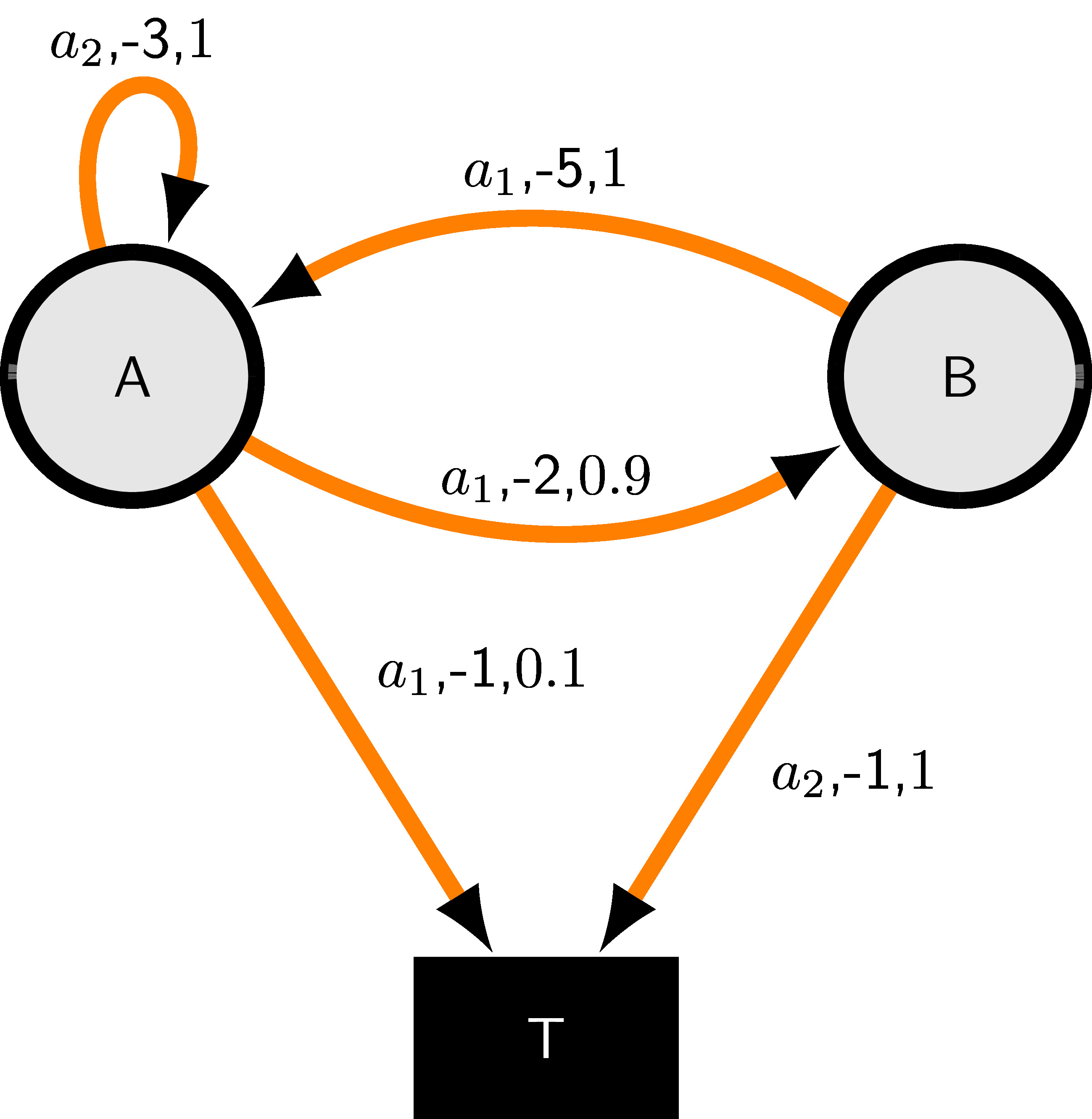
Consider the following policies: \(\pi_1 = (a_1,a_2)\) (i.e., take action \(a_1\) in state \(A\) and \(a_2\) in state \(B\)) and \(\pi_2 = (a_1,a_1)\).

Answer the following:

1. Are \(\pi_1\) and \(\pi_2\) proper?

2. Calculate \(TJ\), \(T_{\pi_1}J\), and \(T_{\pi_2}J\) for \(J = [15,10]\).

Exercise 2.3 The CS6700 mid-term is an open book exam with two questions. For each question, a student taking this exam can either (i) think and solve the problem; or (ii) search the internet for the solution. If he/she chooses to think, then he/she has a probability \(p_1\) of finding the right solution approach. In the case when the right approach is found, the student has a probability \(p_2\) of writing an answer that secures full marks. The corresponding probabilities for option (ii) are \(q_1\) and \(q_2\). The draconian instructor would let the student pass only if both problems are solved perfectly.

Assume \(p_i, q_i >0\), for \(i=1,2\), and answer the following:

1. Formulate this problem as an SSP with the goal of passing the exam, and characterize the optimal policy.

2. Find a suitable condition on \(p_i, q_i\) under which it is optimal to think for each question.

3. When is it optimal to search the internet for each question?

References

Bertsekas, Dimitri P. 2012. Dynamic Programming and Optimal Control, Vol. II, 4th Edition. Athena Scientific.