Chapter 1 Finite horizon model
1.1 A few examples
Example 1.1 (Machine replacement) Consider a machine replacement problem over \(N\) stages. In each stage, the machine can be in one of the \(n\) states, denoted \(\{1,\ldots,n\}\). Let \(g(i)\) denote the cost of operating the machine in state \(i\) in any stage, with \[g(1) \le g(2) \ldots \le g(n).\]
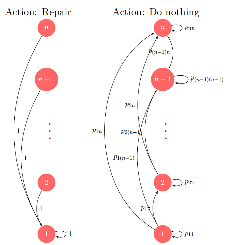
Figure 1.1: Transition diagrams for the two actions in the machine replacement example.
The system is stochastic, with \(p_{ij}\) denoting the probability that the machine goes from state \(i\) to \(j\). Note that the machine can either go worse or stay in the same conditions, which implies \(p_{ij} =0\) for \(j<i\). The state of the machine at the beginning of each stage is known and the possible actions are (i) perform no maintenance, i.e., let the machine run in the current state; and (ii) repair the machine at a cost \(R\). On repair, the machine transitions to state \(1\) and remains there for one stage. The problem is to choose the actions in an optimal manner so that the total cost (summed over \(N\) stages) is minimized. Intuitively, it makes little sense to repair the machine when the stage is close to the final one, and we shall later establish that the decision rule (formalized as policy) that uses a threshold (for the stage) to decide whether to repair or not is optimal.
Example 1.2 (Chess match) A chess player would like to decide on the optimal playing style to win against an opponent in a match that proceeds as follows: Two games are played, with a score of \(1\) for win, \(0\) for loss and \(0.5\) for a draw. If the score is tied at the end of two games, then the players get into a sudden death phase, where first player to win a game secures victory in the match.
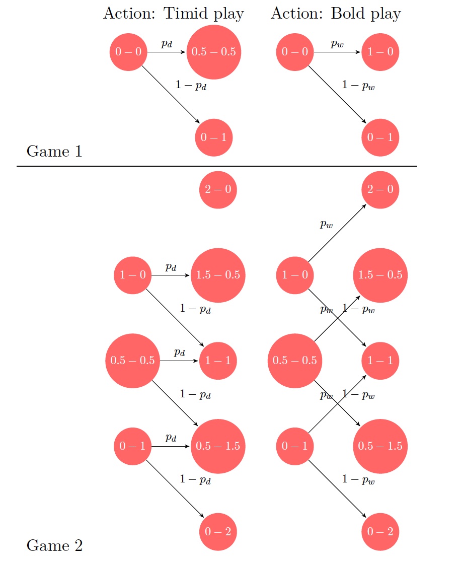
Figure 1.2: Transition diagrams for the two styles of play in the two game chess match example.
Fixing an opponent, the first player (whose style we want to optimize) can either play in a timid or bold fashion in each game. Timid play leads to a draw with probability (w.p.)* \(p_d\) and loss w.p. \((1-p_d)\), while bold play leads to a win w.p. \(p_w\) and loss w.p. \(1-p_w\). It is apparent that in sudden death phase, bold play is optimal and so, the problem is to choose the best playing style in the first two games.
The salient features in each of the examples above are states, actions, costs and transitions between states. These components constitute a Markov decision process and considering that we operate in a multi-stage problem, where the number \(N\) of stages is fixed in advance, the problem is usually referred as an MDP with a “finite horizon”. We formalize this setting next.
1.2 The framework
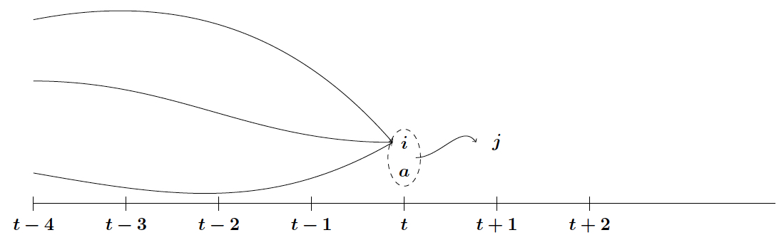
Let \(\mathcal{X}\) denote the state space and \(\mathcal{A}\) the action space, both assumed to be finite. We consider a homogeneous setting, where \(x_k\) (the current state) is in \(\mathcal{X}\), the action \(a_k \in A(x_k) \subset \mathcal{A}\) (In general, the states and actions could be time-dependent). The system is characterized by transition probabilities, given by \[p_{ij}(a) = \mathbb{P}\left[x_{k+1} = j \mid x_k=i, a_k=a\right].\] Notice that the state evolution satisfies the the controlled Markov property, that is
\[\begin{aligned} \mathbb{P}\left[x_{t+1}=j\mid x_t=i,a_t=a,\ldots,x_0=i_0,a_0=b_0\right] = p_{ij}(a), \end{aligned}\]
for any \(i_0,i_1,\ldots, i,j, b_0,b_1\ldots,a\).
Continuing on the MDP formulation, the next component is per-stage cost, given as \(g_k(i,a,j)\). The latter denotes the cost when the system is in state \(i\) and action \(a\) is taken leading to state \(j\), in stage \(k\). There is also a termination cost \(g(x_N)\), with \(x_N\) denoting the state at stage \(N\).
A policy \(\pi\) is a sequence of functions \(\{\mu_0,\ldots, \mu_{N-1}\}\), where \(\mu_k:\mathcal{X}\rightarrow \mathcal{A}\) specifies the action to be taken for every possible state at stage \(k\). A policy is admissible if \(\mu_k(i) \in A(i)\), \(\forall i \in \mathcal{X}\) and \(k=0,\ldots,N-1\). Let \(\Pi\) denote the set of admissible policies.
Given an initial state \(x_0\) and policy \(\pi\), the expected cost (also referred to as value function) is defined as \[\begin{align} J_\pi(x_0) = \mathbb{E}\left[ g_N(x_N) + \sum_{k=0}^{N-1} g_k(x_k, \mu_k(x_k), x_{k+1}]\right], \tag{1.1} \end{align}\] where the expectation is w.r.t. the transition probabilities that govern the state evolution. Notice that, for a fixed policy \(\pi\), the sequence of states visited, say \(\{x_0,\ldots,x_N\}\) forms a Markov chain.
The goal in an MDP is to find a policy, say \(\pi^*\), that optimizes the expected cost, i.e., \[\begin{aligned} J_{\pi^*}(x_0) = \min_{\pi \in \Pi} J_\pi(x_0). \end{aligned}\]
1.3 Open vs. closed loop
Given an MDP, is it strictly necessary to have a policy \(\pi=\{\mu_0,\ldots,\mu_{N-1}\}\), where each \(\mu_k(x_k)\) specifies the action to be taken in the state \(x_k\) at stage k? We shall refer to such policies as closed-loop, since they use the information available through the current state to decide on the next action. An alternative is to fix the sequence of actions, say \(a_0,\ldots,a_{N-1}\) beforehand, which is the open-loop alternative. Intuitively, closed loop cannot hurt and may even be advantageous in stochastic systems, where uncertainty is involved. We shall illustrate the latter claim through the chess match example.
Example 1.3 (Chess match - revisited) Consider the following (exhaustive) list of open-loop policies:
| Game \(1\) | Game \(2\) | Probability of win | |
|---|---|---|---|
| Policy \(\pi_1\) | Timid | Timid | \(p_d^2 p_w\) |
| Policy \(\pi_2\) | Bold | Bold | \(p_w^2 + 2p_w^2(1-p_w)\) |
| Policy \(\pi_3\) | Bold | Timid | \(p_w p_d + p_w^2 (1-p_d)\) |
| Policy \(\pi_4\) | Timid | Bold | \(p_w p_d + p_w^2 (1-p_d)\) |
With policy \(\pi_1\), the match is won only if the two games are drawn and a win happens in sudden death, leading to a probability of match win of \(p_d^2 p_w\). The match win probability for other policies can be calculated using similar arguments. Observe that, \(\pi_3\) and \(\pi_4\) are better than \(\pi_1\), since \(p_w p_d > p_w p_d^2\). On the other hand, a simple calculation shows that \(\pi_2\) is better than \(\pi_1\) when \(3p_w > p_d\). So, ignoring \(\pi_1\), the best open-loop policy calculation is given as \[\begin{aligned} &\max\left( p_w^2(3-2p_w), p_w p_d + p_w^2(1-p_d)\right)\\ &= \max\left( p_w^2+2p_w^2(1-p_w), p_w^2 + p_w p_d(1-p_w)\right)\\ &= p_w^2+p_w(1-p_w) \max(2p_w,p_d). \end{aligned}\]
If \(2p_w <p_d\), then policies \(\pi_3\) and \(\pi_4\) are better than \(\pi_2\), implying that timid play in one of the games is best. In the complementary case, it is better to play bold in both games. With \(p_w = 0.45\) and \(p_d=0.9\), the probability of win turns out to be \(0.425\), which amounts to less than \(50-50\) chance of a match win.
We shall now exhibit a closed loop strategy that can do better the best open-loop policy, even in the case when* \(p_w < 0.5\). Let \(\pi_c\) be a policy that play timid if the player is leading in the score and plays bold otherwise. Then, \[\begin{aligned} \mathbb{P}\left[\textrm{win with } \pi_c\right] &= p_w p_d + p_w\left( p_w(1-p_d) + (1-p_w)p_w\right)\\ & = p_w^2(2-p_w) + p_w(1-p_w)p_d. \end{aligned}\] For the case when \(p_w=0.45\) and \(p_d=0.9\), the probability of match win with \(\pi_c\) turns out to be \(0.53\), i.e., a more than \(50-50\) chance of win, unlike the open-loop alternatives.
1.4 Optimality principle and DP algorithm
Let \(\pi^* = \{\mu_0^*,\mu_1^*,\ldots,\mu_{N-1}^*\}\) denote an optimal policy, i.e., a policy that minimizes the expected cost as defined in (1.1). Consider the following tail sub-problem: \[\begin{align} \min_{\pi^i=\{\mu_i,\ldots,\mu_{N-1}\}} \mathbb{E}\left[ g_N(x_N) + \sum_{k=i}^{N-1} g_k(x_k, \mu_k(x_k), x_{k+1}]\right], \tag{1.2} \end{align}\] The principle of optimality states that the truncated policy \(\{\mu_i^*,\mu_1^*,\ldots,\mu_{N-1}^*\}\) is optimal for the \((N-i)\) stage tail sub=problem in (1.2). A rigorous justification of this claim is available in Section 1.5 of (D. P. Bertsekas 2017).
From the optimality principle, it is intuitively clear that a solution to any tail sub-problem starting at stage \(k\) (see (1.2)) would be useful in arriving at a solution for the tail sub-problem starting at stage \(k-1\). In other words, an approach that solves tail sub-problems by going backwards in time, from \(N-1\) to \(0\) should give the optimal cost, say \(J^*(x_0)\) (corresponding to policy \(\pi^*\) for the original \(N\)-stage problem) at the end. This idea motivates the following algorithm:
Example 1.4 In the machine replacement example, applying DP algorithm would lead to the following recursion: For \(i=1,\ldots,n\), \[\begin{aligned} J_N(i) &= 0, \\ J_k(x_k) &= \min \left(R + g(1) + J_{k+1}(1), g(i) + \sum_{j=i}^n p_{ij} J_{k+1}(j)\right). \end{aligned}\] The first term in the minimum above corresponds to the “repair” action (which transitions the state to \(1\), remaining there for one stage), while the second term corresponds to the “do nothing” action, which can transition the state to some \(j\ge i\), with respective probability \(p_{ij}\).
Next, we establish that the DP algorithm returns the optimal expected cost \(J^*(x_0)\) corresponding to optimal policy \(\pi^*\).
Proposition 1.1 For every \(x_0 \in \mathcal{X}\), the function \(J_0(x_0)\) obtained at the end of DP algorithm coincides with the optimal expected cost \(J^*(x_0)\).
Proof. For any admissible policy \(\pi=\{\mu_0,\ldots,,\mu_{N-1}\}\), let \(\pi^k=\{\mu_k,\ldots,\mu_{N-1}\}\), for \(k=0,1,\ldots, N-1\). Further, let \(J_k^*(x_k)\) denote the optimal cost for the tail sub-problem starting in state \(x_k\) at stage \(k\), i.e., \[\begin{aligned} J_k^*(x_k) = \min_{\pi^k=\{\mu_k,\ldots,\mu_{N-1}\}} \mathbb{E}\left[ g_N(x_N) + \sum_{i=k}^{N-1} g_i(x_i, \mu_i(x_i), x_{i+1}]\right]. \end{aligned}\] We establish the \(J_k^*(x_k) = J_k(x_k)\), for all \(x_k\) and \(k=0,\ldots,N-1\), via induction over the stage \(k\). The first step follows trivially since \(J^*_N(x_N) = g_N(x_N) = J_N(x_N)\). Assume that the following holds: \(J_{k+1}^*(x_{k+1}) = J_{k+1}(x_{k+1})\), for all \(x_{k+1}\) and some \(k\). Then, we have \[\begin{align} J_k^*(x_k) &= \min_{\mu_k,\pi^{k+1}} \mathbb{E}\left[ g_N(x_N) + g_k(x_k,\mu_k(x_k),x_{k+1}) + \sum_{i=k+1}^{N-1} g_i(x_i, \mu_i(x_i), x_{i+1})\right]\\ &= \min_{\mu_k} \mathbb{E}\left[ g_k(x_k,\mu_k(x_k),x_{k+1}) + \min_{\pi^{k+1}} \left[ g_N(x_N) + \sum_{i=k+1}^{N-1} g_i(x_i, \mu_i(x_i), x_{i+1})\right]\right]\\ &= \min_{\mu_k} \mathbb{E}\left[ g_k(x_k,\mu_k(x_k),x_{k+1}) + J_{k+1}^*(x_{k+1})\right]\tag{1.3}\\ &= \min_{\mu_k} \mathbb{E}\left[ g_k(x_k,\mu_k(x_k),x_{k+1}) + J_{k+1}^*(x_{k+1})\right]\tag{1.4}\\ &= \min_{a_k\in A(x_k)} \mathbb{E}\left[ g_k(x_k,a_k,x_{k+1}) + J_{k+1}^*(x_{k+1})\right]\tag{1.5}\\ &=J_k(x_k). \end{align}\] In the above, we used the principle of optimality in (1.3), induction hypothesis in (1.4), and the following equivalence in (1.5): \[\min_{\mu \in B} F(x,\mu(x)) = \min_{a \in A(x)} F(x,a),\] where \(B=\{\mu \mid \mu(x)\in A(x)\}\).
Example 1.5 (Linear system with quadratic cost) A material, at temperature \(x_0\), is passed through two ovens, with temperatures \(a_0\) and \(a_1\), respectively. The final temperature of the material is denoted \(x_2\) and the goal is to get \(x_2\) as close as possible to a target \(T\).*
Suppose that the state evolution is governed by \[\begin{align} x_{k+1} = (1-\alpha) x_k + \alpha a_k, k=0,1. (\#eq:lq-state) \end{align}\] The problem is a deterministic MDP with two stages and the goal is to choose \(a_0, a_1\) so that the following total cost is minimized: \[a_0^2 + a_1^2 + (x_2 - T)^2.\]
Applying the DP algorithm the problem formulated above, we have \[J_2(x_2) = (x_2-T)^2.\] Going backwards, we obtain \[\begin{aligned} J_1(x_1) &= \min_{a_1}\left( a_1^2 + J_2(x_2)\right)\\ &= \min_{a_1}\left( a_1^2 + J_2((1-\alpha) x_1 + \alpha a_1)\right)\\ &= \min_{a_1}\left( a_1^2 + \left((1-\alpha) x_1 + \alpha a_1 - T\right)^2\right), \end{aligned}\] where we used the state equation in the second equality above and the expression for \(J_2(\cdot)\) in the last equality. A straightforward calculation for optimizing \(a_1\) yields \[\begin{aligned} \mu_1^*(x_1) = \frac{\alpha(T-(1-\alpha)x_1)}{1+\alpha^2} \textrm{ and } J_1(x_1) = \frac{((1-\alpha)x_1-T)^2}{1+\alpha^2}. \end{aligned}\] Proceeding in a similar fashion to calculate \(a_0^*\) and \(J_0(x_0)\), we obtain \[\begin{aligned} \mu_0^*(x_0) = \frac{(1-\alpha)\alpha(T-(1-\alpha)^2x_0)}{1+\alpha^2(1+(1-\alpha)^2)} \textrm{ and } J_0(x_0) = \frac{((1-\alpha)^2x_0-T)^2}{1+\alpha^2(1+(1-\alpha)^2)}. \end{aligned}\] Notice that, the optimal action in each stage is linear, and the cost-to-go is quadratic in the state variable and this observation is facilitated by the fact that the state evolution is linear and the single stage cost is quadratic. Further, adding (zero-mean) noise into the equation governing state evolution does not change the optimal action. To see this, let \(w_i, i=1,2\) be zero-mean r.v.s with bounded variance. Let \[x_{k+1} = (1-\alpha) x_k + \alpha a_k + w_k, k=0,1.\] Then, using the DP algorithm, \(J_1(x_1)\) turns out to be \[\begin{aligned} J_1(x_1) &= \min_{a_1}\left( a_1^2 + \left((1-\alpha) x_1 + \alpha a_1 + w_1 - T\right)^2\right)\\ &= \min_{a_1}\left( a_1^2 + \left((1-\alpha) x_1 + \alpha a_1 - T\right)^2 + 2 \mathbb{E}(w_1)\left((1-\alpha) x_1 + \alpha a_1 - T\right) + \mathbb{E}(w_1^2) \right)\\ &= \min_{a_1}\left( a_1^2 + \left((1-\alpha) x_1 + \alpha a_1 - T\right)^2 + \mathbb{E}(w_1^2) \right),\qquad\qquad (\textrm{Since } \mathbb{E}(w_1)=0). \end{aligned}\] It is clear that optimizing \(a_1\) to minimize the RHS above would lead to the same expression as that obtained earlier in the noiseless case. A similar argument works for \(a_0^*\) as well.
Example 1.6 (Chess example - revisited) Consider an extension of the two-game chess match formulated earlier in Example 1.2 to \(N\) games followed by a sudden death phase. Recall that \(p_d\) and \(p_w\) denote the probability of a draw and loss, respectively, for timid and bold play styles. Further, for compactness, the state variable \(x_k\) could be defined to be the net score, i.e., the difference between the number of wins and losses, without any loss of information. Intuitively, before any game, the net score decides the playing style.*
Now, applying DP algorithm after \(k\) games would lead to \[\begin{aligned} J_k(x_k) = \max \bigg( &p_d J_{k+1}(x_k) + (1-p_d) J_{k+1}(x_k - 1),\\ &p_w J_{k+1}(x_k + 1) + (1-p_w) J_{k+1}(x_k - 1) \bigg). \end{aligned}\] The first term in the maximum above corresponds to timid play, which leads to a draw w.p. \(p_d\) (leaving the net score intact) and loss w.p. \((1-p_d)\) (increasing the deficit in the net score by one). The second term, which corresponds to bold playing style, can be understood in a similar fashion. Simplifying the RHS above, it is easy to infer that bold play is optimal if \[\begin{align} \frac{p_w}{p_d} \ge \frac{J_{k+1}(x_k) - J_{k+1}(x_k - 1)}{ J_{k+1}(x_k + 1) - J_{k+1}(x_k - 1)}. (\#eq:condn1) \end{align}\] What remains to be specified is the initial condition, which is given as follows: \[\begin{aligned} J_N(x_N) = \begin{cases} 1 & \textrm{ if } x_N >0,\\ p_w & \textrm{ if } x_N =0,\\ 0 & \textrm{ if } x_N <0. \end{cases} \end{aligned}\] The first (resp. last) case above corresponds to the match being won (resp. lost), implying a setting of \(1\) (resp. \(0\)) for \(J_N(\cdot)\). For the case of a tie (\(x_N=0\)), the match result depends on a win in the sudden death, which occurs w.p. \(p_w\) and hence, \(J_N\) is set to \(p_w\).
Going backwards, \(J_{N-1}\) can be worked out using \(J_N\) and the condition for bold play in @ref\tag{1.6} and the table below specifies \(J_{N-1}\) for all \(x_{N-1}\) (trailing, leading, tied), assuming \(p_d > p_w\).
| \(x_{N-1}\) | \(J_{N-1}(x_{N-1})\) | Best play |
|---|---|---|
| \(>1\) | \(1\) | does not matter |
| \(1\) | \(\max(p_d + (1-p_d)p_w, p_w + (1-p_w)p_w)\) | timid |
| \(= p_d + (1-p_d)p_w\) | ||
| \(0\) | \(p_w\) | bold |
| \(-1\) | \(p_w^2\) | bold |
| \(<-1\) | \(0\) | does not matter |
Interestingly, the values above suggest a playing style that is timid when in the lead and bold play otherwise. The latter policy was shown to do better than any open-loop policy earlier and next, we show that the same claim can be inferred using the DP algorithm by calculating \(J_{N-2}(0)\), i.e., two games to go with a tied score. \[\begin{aligned} J_{N-2}(0) &= \max\left(p_dp_w + (1-p_d)p_w^2, p_w(p_d + (1-p_d)p_w) + (1-p_w)p_w^2 \right)\\ &= p_w(p_w + (p_w+ p_d)(1-p_w), \end{aligned}\] implying that bold play is optimal. As argued before, one could choose \(p_w < 0.5\) and still get better than 50-50 chance of match win whenever \(p_w(p_w + (p_w+ p_d)(1-p_w) > 0.5\).
Example 1.7 (Job scheduling) Suppose there are \(N\) jobs to schedule. Let \(T_i\) be the time it takes for job \(i\) to complete. We assume that \(T_i\) are independent r.v.s. With each job \(i\), there is an associated reward \(R_i\) and completing a job, say \(i\), at time \(t\), would fetch a reward of \(\alpha^t R_i\). Here \(0 < \alpha < 1\) is a discount factor. The goal is to find a schedule for the jobs to maximize the cumulative reward.*
We shall arrive at the optimal schedule via an interchange argument
below. Consider two schedules
\(L = \{i_0,i_1,\ldots,i_{k-1},i,j,i_{k+2},\ldots,i_{N-1}\}\) and
\(L' = \{i_0,i_1,\ldots,i_{k-1},j,i,i_{k+2},\ldots,i_{N-1}\}\). The total
rewards, \(J_L\) and \(J_{L'}\), for these schedules are given by
\[\begin{aligned}
J_L &= \mathbb{E}\left[\alpha^{t_0} R_{i_0} + \ldots + \alpha^{t_{k-1}} R_{i_{k-1}} + \alpha^{t_{k-1}+T_i} R_{i} + \alpha^{t_{k-1}+T_i+T_j} R_{j} + \ldots + \alpha^{t_{N-1}} R_{i_{N-1}} \right],\\
J_{L'} &= \mathbb{E}\left[\alpha^{t_0} R_{i_0} + \ldots + \alpha^{t_{k-1}} R_{i_{k-1}} + \alpha^{t_{k-1}+T_j} R_{j} + \alpha^{t_{k-1}+T_j+T_i} R_{i} + \ldots + \alpha^{t_{N-1}} R_{i_{N-1}} \right].
\end{aligned}\] where \(t_k\) denotes the completion time of job \(i_k\).
Comparing \(J_L\) and \(J_{L'}\), we can infer that \(L\) is better than \(L'\)
if
\[\mathbb{E}\left[\alpha^{t_{k-1}+T_i} R_{i} + \alpha^{t_{k-1}+T_i+T_j} R_{j} \right] \ge \mathbb{E}\left[\alpha^{t_{k-1}+T_j} R_{j} + \alpha^{t_{k-1}+T_i+T_j} R_{i} \right].\]
Using the fact that \(t_{k-1}, T_i, T_j\) are independent, a simple
calculation yields \[\begin{aligned}
\frac{\mathbb{E}\left[\alpha^{T_i}\right] R_{i}}{1- \mathbb{E}\left[\alpha^{T_i}\right]} \ge \frac{\mathbb{E}\left[\alpha^{T_j}\right] R_{j}}{1- \mathbb{E}\left[\alpha^{T_j}\right]}
\end{aligned}\] The inequality above suggests that a policy that
schedules jobs in the order of decreasing
\(\frac{\mathbb{E}\left[\alpha^{T_k}\right] R_{k}}{1- \mathbb{E}\left[\alpha^{T_k}\right]}\)
is optimal.
The discrete time MDPs that we have been analyzing in a finite horizon setting can also be formulated alternatively as follows: \[x_{k+1} = f(x_k,a_k,w_k),\] where \(w_k\) is the source of randomness and is usually referred to as a “disturbance” term. The disturbances \(w_k\) could be i.i.d. or be dependent on \(x_k, a_k\). Such a formulation is more general in the sense that \(x_k\) could take values in an infinite set, for e.g., \(x_k\) is a \(d\)-dimensional real variable. On the other hand, in the case when \(x_k\) takes values in a discrete set, say \(\{1,\ldots,n\}\), then an equivalent formulation for the MDP is to specify the transition probabilities, i.e., \[p_{ij}^a=\mathbb{P}\left[x_{k+1}=j\mid x_k=i,a_k=a\right].\]
We illustrate the formulation using disturbances in a simpler i.i.d. setting. More importantly, the example is used to demonstrate an optimal policy that is based on certain thresholds.
Example 1.8 (Asset selling) Suppose an asset is to be sold and \(w_0,\ldots,w_{N-1}\) are the offers that arrive over \(N\) stages. Assume that \(w_k\) are i.i.d., with a finite mean. In any stage \(k\), the actions available are \(a^1\) and \(a^2\), with \(a^1\) denoting the choice to sell the asset and \(a^2\) the choice to not sell (and wait for a better offer). The problem can be cast into a finite horizon MDP using an additional state, say \(T\) as follows: \[\begin{aligned} x_{k+1} = f(x_k,a_k,w_k), \textrm{ where } f(x_k,a_k,w_k) = \begin{cases} T & \textrm{ if } x_k = T \textrm{ or } (x_k \ne T, a_k = a^1),\\ w_k & \textrm{ if } x_k \ne T, a_k=a^2. \end{cases} \end{aligned}\] The goal is to choose actions to maximize the following total reward objective: \[\begin{aligned} &\mathbb{E}\left[ g_N(x_N) + \sum_{k=0}^{N-1} g_k(x_k,a_k,w_k) \right], \textrm{ where }\\ &g_N(x_N) = \begin{cases} x_N & \textrm{ if } x_N \ne T ,\\ 0 & \textrm{ otherwise }, \end{cases} \textrm{ and }\\ &g_k(x_k,a_k,w_k) = \begin{cases} (1+r)^{N-k} x_k & \textrm{ if } x_k \ne T, a_k = a^1,\\ 0 & \textrm{ otherwise}. \end{cases} \end{aligned}\] In the above, the expectation is w.r.t. \(w_0,\ldots,w_{N-1}\). The rationale behind \(g_k(\cdot,\cdot,\cdot)\) is that selling an asset at \(x_k\) in stage \(k\) would allow an accumulation of interest at rate \(r>0\) for the rest of the \(N-k\) stages.*
Applying the DP algorithm leads to \[\begin{aligned} J_N(x_N) &= g_N(x_N), \\ J_k(x_k) &= \max_{a^1,a^2} \mathbb{E}\left(g_k(x_k,a_k,w_k) + J_{k+1}(x_{k+1})\right)\\ &= \begin{cases} \max\left( (1+r)^{N-k}x_k, \mathbb{E}\left(J_{k+1}(w_k)\right)\right) & \textrm{ if } x_k \ne T,\\ 0 & \textrm{ otherwise}. \end{cases} \end{aligned}\] For the last equality above, we have used the fact that \(x_{k+1} = w_k\) when \(x_k \ne T\).
For notational convenience, let \(V_k(x_k) = \frac{J_k(x_k)}{(1+r)^{N-k}}\) when \(x_k \ne T\). Then, the DP algorithm can be re-written as follows: \[\begin{aligned} V_N(x_N) &= x_N, \\ V_k(x_k) &= \max\left( x_k, \frac{\mathbb{E}\left(V_{k+1}(w_k)\right)}{(1+r)}\right). \end{aligned}\] In the above, the expectation is w.r.t. \(w_k\). Using the fact that \(w_k\) are i.i.d. and letting \(\alpha_k = \frac{\mathbb{E}\left(V_{k+1}(w)\right)}{(1+r)}\), it is easy to see that the optimal policy is to sell if \(x_k \ge \alpha_k\) and not sell in the complementary case, i.e., \[\begin{aligned} \mu_k^*(x_k) =\begin{cases} a^1 & \textrm{ if } x_k \ge \alpha_k,\\ a^2 & \textrm{ otherwise}. \end{cases} \end{aligned}\] We now claim that \(\alpha_k \ge \alpha_{k+1}\). To establish this claim, it is enough to show that \(V_k(x) \ge V_{k+1}(x), \forall x\). For the case when \(k=N-1\), observe that \[\begin{aligned} V_{N-1}(x) = \max\left( x, \frac{\mathbb{E}\left(V_{N}(w)\right)}{(1+r)}\right) = \max\left( x, \frac{\mathbb{E}\left(w\right)}{(1+r)}\right) \ge x = V_N(x). \end{aligned}\] For \(k=N-2\), \[\begin{aligned} V_{N-2}(x) = \max\left( x, \frac{\mathbb{E}\left(V_{N-1}(w)\right)}{(1+r)}\right) \ge \max\left( x, \frac{\mathbb{E}\left(V_N(w)\right)}{(1+r)}\right) = V_{N-1}(x). \end{aligned}\] Proceeding similarly, we have \(V_k(x) \ge V_{k+1}(x)\), \(\forall x, \forall k\).
For simplicity, assume \(w\) is a positive-valued continuous r.v. with distribution \(F_w\) and density \(h\). Then, using \(V_{k+1}(w) = \begin{cases} w & \textrm{ if } \alpha_{k+1} \le w,\\ \alpha_{k+1} & \textrm{ otherwise.} \end{cases}\), we have \[\begin{align} \alpha_k &= \frac{\mathbb{E}\left(V_{k+1}(w)\right)}{(1+r)} \\ &= \frac{1}{(1+r)} \int V_{k+1}(w) h(w) dw \\ & =\frac{1}{(1+r)} \int_0^{\alpha_{k+1}} \alpha_{k+1} h(w) dw + \frac{1}{(1+r)} \int_{\alpha_{k+1}}^\infty w h(w) dw\\ & =\frac{\alpha_{k+1} F_w(\alpha_{k+1})}{(1+r)} + \frac{1}{(1+r)} \int_{\alpha_{k+1}}^\infty w h(w) dw (\#eq:t122)\\ & \le \frac{\alpha_{k+1}}{(1+r)} + \frac{1}{(1+r)} \int_{0}^\infty w h(w) dw\\ & = \frac{\alpha_{k+1}}{(1+r)} + \frac{E(w)}{(1+r)}, \end{align}\] where the last equality follows since \(w\) is positive. From the foregoing, we have \[0 \le \alpha_k \le \frac{E(w)}{r}.\] Since \(\alpha_{k+1} \le \alpha_{k}\), the sequence \(\{\alpha_k\}\) converges as \(k\rightarrow -\infty\) to some \(\bar\alpha \in \left[0,\frac{\mathbb{E}(w)}{(1+r)}\right]\). Further, taking limits as \(k \rightarrow -\infty\) in @ref\tag{1.7}, and using the left continuity of \(F_w\), we obtain \[\begin{aligned} \bar \alpha & =\frac{\bar\alpha F_w(\bar\alpha)}{(1+r)} + \frac{1}{(1+r)} \int_{\bar\alpha}^\infty w h(w) dw. \end{aligned}\] If the horizon \(N\) is large, then an approximation to the optimal policy is \[\begin{aligned} \mu^*(x_k) =\begin{cases} a^1 & \textrm{ if } x_k \ge \bar\alpha,\\ a^2 & \textrm{ otherwise}. \end{cases} \end{aligned}\]
1.5 Exercises
Exercise 1.1 A finite horizon MDP setting is as follows:
Horizon \(N=2\), states \(\{1,2\}\) and actions \(\{a,b\}\) (available in each state).
Transition probabilities are given by \[\begin{aligned} p_{11}(a)=p_{12}(a)=\frac{1}{2};\quad p_{11}(b)=\frac{1}{4}, p_{12}(b)=\frac{3}{4};\\ p_{21}(a)=\frac{2}{3},p_{22}(a)=\frac{1}{3};\quad p_{21}(b)=\frac{1}{3}, p_{22}(b)=\frac{2}{3}; \end{aligned}\] The time-invariant single-stage costs are as follows: \[\begin{aligned} g(1,a)=3, g(1,b)=4, g(2,a)=2, g(2,b)=1. \end{aligned}\] There is no terminal cost. Calculate the optimal expected cost using the DP algorithm and specify an optimal policy.
Exercise 1.2 Consider a finite horizon MDP with \(N\) stages. Suppose there \(n\) possible states in each stage and \(m\) actions in each state. Why is the DP algorithm computationally less intensive as compared to an approach that calculates the expected cost \(J^\pi\) for each policy \(\pi\)? Argue using the number of operations required for both algorithms, as a function of \(m,n\) and \(N\).
Exercise 1.3 Consider the finite horizon MDP setting. In place of the expected cost objective defined there, consider the following alternative cost objective for any policy \(\pi\) and initial state \(x_0\): \[\begin{aligned} J_\pi(x_0) = \mathbb{E}\left[ \exp\left( g_N(x_N) + \sum_{k=0}^{N-1} g_k(x_k, \mu_k(x_k), x_{k+1}]\right)\right], \end{aligned}\]
Answer the following:
Show that an optimal cost and an optimal policy can be obtained by the following DP-algorithm variant: \[\begin{aligned} J_N(x_N) &= \exp\left(g_N(x_N)\right), \\ J_k(x_k) &= \min_{a_k \in A(x_k)} \mathbb{E}_{x_{k+1}} \left(\exp\left(g_k(x_k,a_k,x_{k+1})\right) J_{k+1}(x_{k+1}) \right). \end{aligned}\]
Let \(V_k(x_k) = \log J_k(x_k)\). Assume that the single stage cost \(g_k\) is a function of \(x_k\) and \(a_k\) only (and does not depend on \(x_{k+1}\)). Then, show that the DP algorithm, which is specified above, can be re-written as \[\begin{aligned} V_N(x_N) &= g_N(x_N), \\ v_k(x_k) &= \min_{a_k \in A(x_k)} \left(g_k(x_k,a_k) + \log \mathbb{E}_{x_{k+1}} \left(\exp\left(V_{k+1}(x_{k+1}\right)\right) \right). \end{aligned}\]
Recall the "oven problem" which was a linear system with quadratic cost problem over two stages. Using the notation from this problem, consider the following ‘exponentiated cost’ objective: For a given scalar \(\theta\), define \[\begin{align} J_{a_0,a_1}(x_0) &= \mathbb{E}\left[ \exp\left(\theta\left( a_0^2 + a_1^2 + (x_2 - T)^2\right)\right)\right], \tag{1.8} \end{align}\] where \[x_{k+1} = (1-\alpha)x_k + \alpha a_k + w_k, \textrm{ for } k=0,1.\] In the above, \(w_k\) is a Gaussian random variable with mean zero and variance \(\sigma^2\).
Solve problem (1.8) using the DP algorithm from the part above. Identify the optimal policy, and the optimal expected ‘exponentiated’ cost.
Exercise 1.4 A machine is either running or broken. If it runs for a week, it makes a profit of \(1000\) INR, while the profit is zero if it fails during the week. For a machine that is running at the start of a week, we could perform preventive maintenance at the cost of \(200\) INR, and the probability of machine failing during the week is \(0.4\). In case the preventive maintenance is not performed, the failure probability is \(0.7\). A machine that is broken at the start of a week can be repaired at a cost of \(400\) INR, in which case the machine would fail with probability \(0.4\), or replaced at a cost of \(1500\) INR. A replaced machine is guaranteed to run through its first week.
Answer the following:
Formulate this problem as an MDP with the goal of maximizing profit for a given number of weeks.
Find the optimal repair/replace/maintenance policy under a horizon of four weeks, assuming a new machine at the start of the first week.
Exercise 1.5 You are walking along a line of \(N\) stores in a shopping complex, looking to buy food before entering a movie hall at the end of the store line. Each store along the line has a probabi1ity \(p\) of providing the food you like. You cannot see what the next store (say \(k+1\)) offers, while you are at the \(k\)th store and once you pass store \(k\), you cannot return to it. You can choose to buy at store \(k\), if it has the food item you like and pay an amount \(N-k\) (since you have to carry this item for a distance proportional to \(N-k\)). If you pass through all the stores without buying, then you have to pay \(\frac{1}{1-p}\) at the entrance to the movie hall to get some food.
Answer the following:
Formulate this problem as a finite horizon MDP.
Write a DP algorithm for solving the problem.
Characterize the optimal policy as best as you can. This may be done with or without the DP algorithm.
Hint: Follow the technique from the asset selling example, since the question is about when to stop. Argue that if it is optimal to buy at store \(k\) when the item you like is available, then it is optimal to buy at store \(k+1\) when the likeable food is available there. Show that \(\mathbb{E}\left( J_{k+1}(x)\right)\) is a constant that depends on \(n-k\), leading to an optimal threshold-based policy.
Exercise 1.6 Suppose there are \(N\) jobs to schedule on a computer. Let \(T_i\) be the time it takes for job \(i\) to complete. Here \(T_i\) is a positive scalar. When job \(i\) is scheduled, with probability \(p_i\) a portion \(\beta_i\) (a positive scalar) of its execution time \(T_i\) is completed and with probability \((1-p_i)\), the computer crashes (not allowing any more job runs). Find the optimal schedule for the jobs, so that the total proportion of jobs completed is maximal.
Hint: Use an interchange argument to show that it is optimal to schedule jobs in the order \(\dfrac{p_i\beta_i Z_i}{1-p_i}\), where \(Z_i\) is the residual execution time of job \(i \in \{1,\ldots,N\}\).
Exercise 1.7 Consider a finite horizon MDP setting, where the single stage cost is time-invariant, i.e., \(g_k \equiv g\), \(\forall k\). Also, assume that the same set of states and actions are available in each stage.
Answer the following:
If \(J_{N-1}(x) \le J_N(x)\) for all \(x\in\mathcal{X}\), then, \[J_{k}(x) \le J_{k+1}(x), \textrm{ for all } x \in \mathcal{X}, \textrm{ and } k.\]
If \(J_{N-1}(x) \ge J_N(x)\) for all \(x\in\mathcal{X}\), then, \[J_{k}(x) \ge J_{k+1}(x), \textrm{ for all } x \in \mathcal{X}, \textrm{ and } k.\]
Exercise 1.8 Suppose that the course notes for CS6700 has been written up and the number of errors in this document is \(X\) (a non-negative scalar). Assume that there are \(N\) students willing to proofread the notes. The proofreading exercise proceeds in a serial fashion, with each student charging the same amount, say \(c_1>0\). The \(k\)th student can find an error in the notes with probabi1ity \(p_k\), and this is independent of the number of errors found by previous students. The course instructor has an option to stop proofreading and publish the notes or continue proofreading. Each undetected error in the published notes costs \(c_2>0\).
Answer the following:
Formulate this problem as a finite horizon MDP.
Write a DP algorithm for solving the problem.
Analyze the DP algorithm to characterize as best as you can the optimal selling policy.
Discuss the modifications to the DP algorithm for the case when the number of errors \(X\) is a r.v.